
Do not index
Canonical URL
Data drift methods are excellent tools for understanding changes in feature distributions over time. However, they are often misused with the intention of detecting model failures directly. Just by looking at raw drift results, it is impossible to tell how a feature’s drift would affect a model's performance.
But, what if we use drift signals as inputs of a more complex method to try to estimate the model's performance?
In this experiment, we will give data drift methods a second chance and try to take the best out of them. We will build a technique that relies on drift signals to estimate model performance and compare its results against the current SoTA performance estimation methods to see which technique performs best.
Experiment Setup
To effectively compare data drift signals against performance estimation methods, we designed an evaluation framework that emulates a typical production ML model and ran multiple dataset-model experiments.
By 'typical production ML model,' we mean that we will have a training dataset, a test set—which, apart from evaluating the monitored model, we will use to establish a reference for the data drift and performance estimation methods—and a production dataset—which will be data that was unseen by the model and will be used to evaluate the results of the data drift signal models and performance estimation methods.
To make sure the results are not biased, we trained different types of models for multiple prediction tasks. This means we will run multiple experiments, and in each of them, we will do four things:
For that reason, we will run multiple experiments, and in each of them, we will do four things:
- Separate the first year of data in each dataset and use it as a training period.
- Fit three commonly used binary classification algorithms on the training data: Logistic Regression, Random Forest, and LightGBM.
- The trained models were used to predict labels on the remaining part of the dataset, which was divided into two periods: reference and production.
- Apply all the proposed benchmarks to estimate the performance of the ML models during the production period.
- Collect results and evaluate them.
Datasets and Models
We used datasets from the Folktables package. Folktables preprocesses US census data to create a set of binary classification problems.
We use the following tasks: ACSIncome, ACSMobility, ACSEmployment, ACSTravelTime, and ACSPublicCoverage. For each of these five prediction tasks, we fetch Folktables data for all 50 US states spanning four consecutive years (2015-2018), giving us 250 datasets with which to experiment.
For each of those 250 datasets, we trained a Logistic Regressor, a Random Forest Classifier, and a LightGBM Classifier, giving us 750 dataset-model pairs.
We then filtered out models that performed poorly at test time (ROC_AUC < 0.6) and datasets with three or fewer chunks for reference. This was done for a couple of reasons: first, we don't expect that a model with a test ROC_AUC score lower than 0.6 would ever get to production, so we are not interested in measuring how the methods would perform on these types of models; and second, we removed models that had very few chunks for reference because that would mean that the drift signals and performance estimation methods would have very little data to be fitted on.
These changes gave us a total of 580 dataset-model pairs to evaluate the following performance estimation methods.
Chunks are data samples where monitoring calculations are performed; in our experiments, each chunk had 2000 observations.
Methods
Test set performance
Data scientists generally assume that test set performance is representative of production performance unless there's significant data drift. For this reason, test set performance is the simplest form of performance estimation.
This benchmark assumes that the model's performance on the production data is constant and equal to the performance calculated on the test set.
Data drift signals for performance estimation (DriftSignal Model)
This method uses univariate and multivariate data drift information as features of a DriftSignal model to estimate the performance of the model we monitor.
The method works as follows:
- Fit univariate/multivariate drift detection calculator on reference data (test set).
- Take the fitted calculators to measure the observed drift in the production set. For univariate drift detection methods, we use Jensen Shannon, Kolmogorov-Smirnov, and Chi2 distance metrics/tests. Meanwhile, we use the PCA Reconstruction Error and Domain Classifier for multivariate methods.
- Build a DriftSignal model that trains a regression algorithm using the drift results from the reference period as features and the monitored model performance as a target.
- Estimate the performance of the monitored model on the production set using the trained DriftSignal model.
If you are curious about the full implementation of this method, open this toggle or check out its GitHub Gist.
import numpy as np
import nannyml as nml
import pandas as pd

class DriftSignalsModel:
    def __init__(
        self,
        y_pred_proba,
        y_pred,
        y_true,
        features,
        treat_as_cat,
        metric,
        regressor,
        cat_methods=['jensen_shannon'],
        cont_methods=['jensen_shannon'],
        method_type='both',
        problem_type='classification_binary',
        chunk_size=2000,
        ):

        self.y_pred_proba = y_pred_proba
        self.y_pred = y_pred
        self.y_true = y_true
        self.features = features
        self.treat_as_cat = treat_as_cat
        self.metric = metric
        self.regressor = regressor
        self.cat_methods = cat_methods
        self.cont_methods = cont_methods
        self.method_type = method_type
        self.problem_type = problem_type
        self.chunk_size = chunk_size

    def fit_calculators(self, reference):
        drift_signals = []

        if self.method_type == 'univariate' or self.method_type == 'both':
            # Univariate drift
            self.uni_calc = nml.UnivariateDriftCalculator(
                column_names=self.features,
                continuous_methods=self.cont_methods,
                categorical_methods=self.cat_methods,
                treat_as_categorical=self.treat_as_cat,
                chunk_size=self.chunk_size
            )
            self.uni_calc.fit(reference)

            uni_drift_signals_df = self.uni_calc.result.to_df(multilevel=False)
            continuous_columns = list(set(self.features).difference(self.treat_as_cat))
            continuous_uni_drift_columns = [column_name + f'_{distance_metric}_value' for column_name in continuous_columns for distance_metric in self.cont_methods]
            categorical_uni_drift_columns = [column_name + f'_{distance_metric}_value' for column_name in self.treat_as_cat for distance_metric in self.cat_methods]
            uni_drift_columns = continuous_uni_drift_columns + categorical_uni_drift_columns

            if self.method_type == 'univariate':
                uni_drift_columns.append('chunk_period')
            drift_signals.append(uni_drift_signals_df[uni_drift_columns])

        if self.method_type == 'multivariate' or self.method_type == 'both':
            # Data reconstruction error
            self.data_recostruction_calc = nml.DataReconstructionDriftCalculator(
                column_names=self.features,
                chunk_size=self.chunk_size)
            self.data_recostruction_calc.fit(reference)

            reconstruction_error_results_df = self.data_recostruction_calc.result.to_df(multilevel=False)
            reconstruction_error_column = 'reconstruction_error_value'
            drift_signals.append(reconstruction_error_results_df[reconstruction_error_column])

            # Domain classifier
            self.dm_calc = nml.DomainClassifierCalculator(
                feature_column_names=self.features,
                treat_as_categorical=self.treat_as_cat,
                chunk_size=self.chunk_size
            )
            self.dm_calc.fit(reference)

            domain_clf_results_df = self.dm_calc.result.to_df(multilevel=False)
            domain_clf_column = 'domain_classifier_auroc_value'
            drift_signals.append(domain_clf_results_df[[domain_clf_column, 'chunk_period']])

        # Realized performance (this will be the y_true of the drift signal models)
        self.performance_calc = nml.PerformanceCalculator(
            y_pred_proba=self.y_pred_proba,
            y_pred=self.y_pred,
            y_true=self.y_true,
            problem_type=self.problem_type,
            metrics=self.metric,
            chunk_size=self.chunk_size)
        self.performance_calc.fit(reference)

        performance_results_df = self.performance_calc.result.to_df(multilevel=False)
        performance_column = self.metric + '_value'

        drift_signals_df = pd.concat(drift_signals, axis=1)
        drif_signals_reference_X = drift_signals_df[drift_signals_df['chunk_period'] == 'reference'].drop(columns='chunk_period')
        drif_signals_reference_y = performance_results_df[performance_results_df['chunk_period'] == 'reference'][performance_column]

        return drif_signals_reference_X, drif_signals_reference_y


    def fit(self, df_reference):
        self.reference = df_reference
        drif_signals_reference_X, drif_signals_reference_y = self.fit_calculators(self.reference)
        self.signals_model = self.regressor.fit(drif_signals_reference_X, drif_signals_reference_y)

    def estimate(self, chunk):
        drift_signals = []
        if self.method_type == 'univariate' or self.method_type == 'both':
            uni_drift_signals = self.uni_calc.calculate(chunk)
            uni_drift_signals_df = uni_drift_signals.to_df(multilevel=False)

            continuous_columns = list(set(self.features).difference(self.treat_as_cat))
            continuous_uni_drift_columns = [column_name + f'_{distance_metric}_value' for column_name in continuous_columns for distance_metric in self.cont_methods]
            categorical_uni_drift_columns = [column_name + f'_{distance_metric}_value' for column_name in self.treat_as_cat for distance_metric in self.cat_methods]
            uni_drift_columns = continuous_uni_drift_columns + categorical_uni_drift_columns

            if self.method_type == 'univariate':
                uni_drift_columns.append('chunk_period')
            drift_signals.append(uni_drift_signals_df[uni_drift_columns])

        if self.method_type == 'multivariate' or self.method_type == 'both':
            reconstruction_error_results = self.data_recostruction_calc.calculate(chunk)
            reconstruction_error_results_df = reconstruction_error_results.to_df(multilevel=False)
            reconstruction_error_column = 'reconstruction_error_value'
            drift_signals.append(reconstruction_error_results_df[reconstruction_error_column])

            domain_clf_results = self.dm_calc.calculate(chunk)
            domain_clf_results_df = domain_clf_results.to_df(multilevel=False)
            domain_clf_column = 'domain_classifier_auroc_value'
            drift_signals.append(domain_clf_results_df[[domain_clf_column, 'chunk_period']])

        drift_signals_df = pd.concat(drift_signals, axis=1)
        drif_signals_chunk_X = drift_signals_df[drift_signals_df['chunk_period'] == 'analysis'].drop(columns='chunk_period')
        estimated_performance = self.signals_model.predict(drif_signals_chunk_X)

        return estimated_performance
Confidence-based Performance Estimation (CBPE)
Generally, when a machine learning classifier returns a prediction, it also provides a numerical value between 0 and 1. This number is often called model score or predicted probability, and it is a way for the model to express its certainty about what class the input data belongs to.
Depending on the model type, these scores can't always be interpreted as probabilities. But by using calibration, we can transform them into real probabilities and use them to estimate the probability of making an error.
For instance, a high-performing model for a large set of observations returns a prediction of 1 (positive class) with a probability of 0.9. This means the model is correct for approximately 90% of these observations, while it is wrong for the other 10%.
CBPE leverages the calibrated confidence scores of the predictions to estimate all the confusion matrix elements (TP, TN, FP, FN) and, with them, estimate any classification performance metric.
We created and open-sourced this method in 2021. For a full explanation of how CBPE works, check out NannyML's documentation.
Probabilistic Adaptive Performance Estimation (PAPE)
PAPE is the latest performance estimation algorithm; we introduced it in mid-2024; our findings show that PAPE outperforms other methodologies, including CBPE, making it the current SoTA method for estimating the performance of classification models. Experimental results show that PAPE is about 10-30% more accurate at estimating model performance than CBPE.
PAPE's algorithm is very similar to CBPE's, but instead, it uses DRE (density ratio estimation) to calibrate the probabilities, considering the current chunk data distribution. In contrast, CBPE calibrates the model only once by looking at the entire reference input distribution, so it misses second-order effects that are crucial for more accurate performance estimation results.
Check out PAPE's paper: Estimating model performance under covariate shift without labels to learn more about it.
Evaluation
Performance estimation is a regression problem. This leads to evaluation metrics such as mean absolute error (MAE) or root mean squared error (RMSE). However, the MAE/RMSE of all data chunks from multiple evaluation cases is meaningless. A large MAE for an evaluation case where the model's performance has a large variance might still be satisfactory. On the other hand, in cases where the model performance is very stable, even small changes (in the absolute scale) in performance might be significant.
To account for this, we scale absolute/squared errors by the standard error (SE) calculated for each evaluation case. We call the SE-scaled metrics mean absolute standard error (MASTE).
- where is the evaluation case index ranging from to , and is the index of the production data chunk ranging from to (number of production chunks in a case ).
- and are respectively realized and estimated performance for case and chunk .
- is the standard error of the evaluation case.
Results
Each performance estimation method tries to estimate the roc_auc of the monitored model. For this reason, we report the MASTE between the estimated and realized roc_auc.
We see that PAPE is the most accurate method, followed by CBPE. Surprisingly, constant test set performance is the third best. This is closely followed by random forest versions of univariate and multivariate drift signal models.
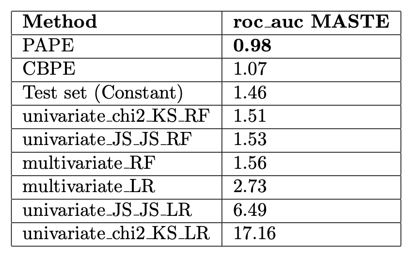
MASTE for roc_auc of the evaluated performance estimation methods. (The smaller, the better).
The following plot shows the quality of performance estimation among different methods, including PAPE and CBPE.
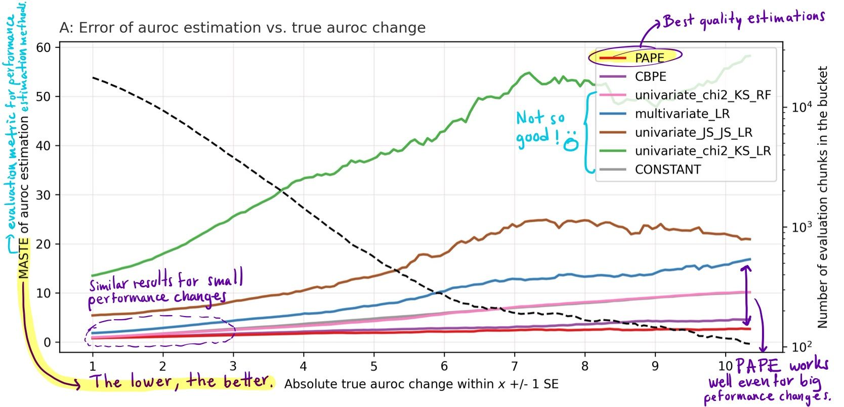
Quality of performance estimation (MASTE of roc_auc) vs absolute performance change (SE). (The lower, the better).
Understanding this plot
- The horizontal axis indicates the centre of the data bucket; for example, value 1 indicates a bucket containing data chunks for which the absolute performance change was in the range of 0-2 performance metric in the Standard Error (SE) unit.
- The left vertical axis shows the Mean Absolute Standard Error (MASTE) of the evaluated method for the data bucket. The right vertical axis indicates the number of data chunks in each bucket on a logarithmic scale.
- In red, PAPE shows the best quality of estimations in the whole evaluated region. It gets significantly better than other methods for large true performance changes.
- In purple, CBPE, the former state-of-the-art method, behaves slightly worse than PAPE.
- Other methods, including univariate and multivariate drift signal models, performed worse than PAPE and CBPE.
- These findings represent aggregated results from experiments across the 580 dataset-model pairs.
Here is a specific time series plot of a model's realized ROC AUC (black) compared against all the performance estimation methods. We see how PAPE (red) accurately estimates the direction of the most significant performance change and closely approximates the magnitude.
.png)
Time series plot of realized vs estimated roc_auc for dataset ACSIncome (California) and LigthGBM model.
Conclusion
Our experiments suggest that there are better tools for detecting performance degradation than data drift, even though we tried our best to extract all the meaningful information from drift signals to create an accurate performance estimation method.
We found that our methods (PAPE and CBPE) are the best approaches for quantifying the impact of data drift on model performance.
Check out PAPE's paper, where we show how PAPE significantly outperforms other existing methods across multiple metrics.
If you want to try out PAPE for free, check out NannyML Cloud, it is available on Azure and AWS.
Written by
