How to Detect Data Drift with Hypothesis Testing

Do not index

Canonical URL

Data drift is a concern to anyone with a machine learning model serving live predictions. The world changes, and as the consumers’ tastes or demographics shift, the model starts receiving feature values different from what it has seen in training, which may result in unexpected outputs.

Detecting feature drift appears to be simple: we just need to decide whether the training and serving distributions of the feature in question are the same or not. There are statistical tests for this, right? Well, there are, but are you sure you are using them correctly?

Univariate drift detection

Monitoring the post-deployment performance of a machine learning model is a crucial part of its life cycle. As the world changes and the data drifts, many models tend to show diminishing performance over time. The best approach to staying alert is to calculate the performance metrics in real-time or to estimate them when the ground truth is not available.

A likely cause of an observed degraded performance is data drift. Data drift is a change in the distribution of the model’s inputs between training and production data. Detecting and analyzing the nature of data drift can help to bring a degraded model back on track. With respect to how (and how many) features are affected, data drift can take one of two forms: one should distinguish between multivariate and univariate data drift.

Multivariate drift is a situation in which the distributions of the individual features don’t necessarily change, but their joint distribution does. It’s tricky to spot since observing each model feature in isolation will not uncover it. If you are interested in detecting multivariate drift, check out this piece on how to do it based on PCA reconstruction errors.

Today, we focus on univariate data drift, a scenario in which the distribution of one or more features shifts in the live production environment compared to what it was in the model’s training data.

Univariate data drift seems to be the simpler to detect of the two: you don’t need to account for complex statistical relationships between multiple variables. Rather, for each of the features, you simply compare two data samples — training and serving — to check whether they are distributed in a similar fashion. Let’s take a look at how this is typically performed in a hypothesis testing framework.

Hypothesis Testing Primer

To keep things concrete, let’s focus on the chi-squared test, frequently used to compare the distributions of categorical variables. The chi-squared test finds widespread application in A/B/C testing, where it is used to verify whether users subjected to different treatments (e.g. are shown advertisement A, B, or C) show different behavior patterns (e.g. purchase frequency).

The same test is often applied in univariate data drift detection to check if a categorical variable measured in two regimes (training and serving, which correspond to purchase and non-purchase in the marketing setting) shows the same category frequencies. If it doesn’t, the data might have drifted. Let’s take a look at a specific example.

Imagine a machine learning model responsible for suggesting content to your users. Let’s assume that one of the model inputs is the user’s device. Let the device be a categorical variable with two categories: desktop and mobile. Here are the category counts from the training and serving data.

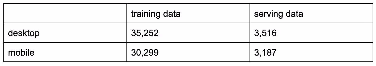
Since the serving sample is much smaller than the training set, let’s express the category counts as relative frequencies for easier comparison.

The category frequencies are definitely very similar between the training and serving sets but they are not exactly the same. Naturally, due to random sampling, we rarely observe the exact same frequencies even in the absence of data drift.

And so the question becomes: are the differences in class frequencies we observed caused by random sampling variation, or by the structural shift in the device variable? The latter would mean we are dealing with data drift.

In order to answer this question, we can employ the statistical hypothesis testing framework.

Chi-2 test

We start by defining the hypotheses, namely two of them. The null hypothesis claims that the differences between training and serving we observed are caused by random chance alone — both samples of data come from the same underlying distribution (population). The alternative hypothesis, on the other hand, claims that the differences are not driven by randomness but rather are caused by data drift.

H₀: Training/serving differences are a result of random noise. H₁: Training/serving differences are a result of data drift.

We will now use the data to test the null hypothesis. If we can reject it, we will state that data drift has happened. If we can’t, we’ll say that since the differences could have been produced by random chance, there is no evidence for the presence of data drift.

The traditional testing approach in our case relies on the fact that under the null hypothesis, a certain quantity is known to follow the chi-2 distribution. This quantity is fittingly referred to as the chi-2 statistic.

Chi-2 statistic

The chi-2 statistic is defined as the normalized sum of squared differences between the expected and observed frequencies. Let’s unpack this statement now.

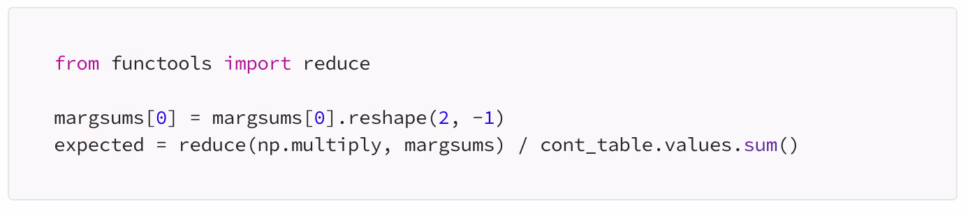
The expected frequencies are what we would have observed under the null hypothesis of no data drift. They are defined as the marginal sums of the contingency table multiplied by each other and scaled by the total count.

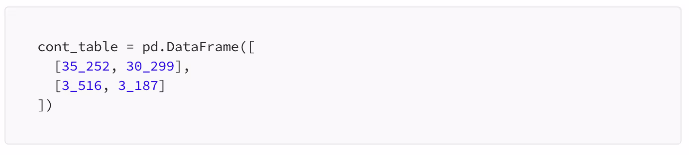
The following contingency table represents the frequencies of our device variable for testing and serving data as defined before.

We can then calculate the marginal sums along both axes as follows.

Finally, we multiply them (we need to transpose the first element to make the multiplication possible) and scale by the global sum.

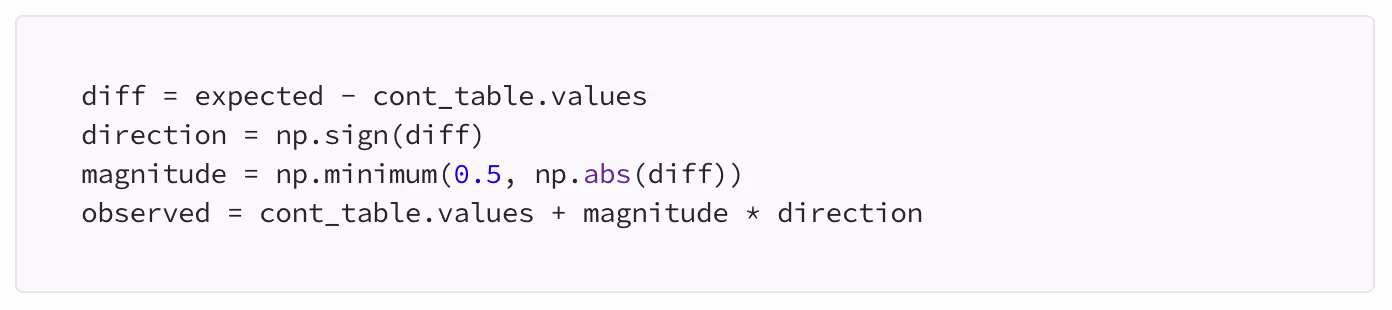
In our special case with only two categories of the variable under test, the test will have just one degree of freedom. This calls for an adjustment of the observed values known as Yates’ correction for continuity. With more categories, you can skip the following four lines of code.

Knowing the expected values, we can calculate the chi-2 statistic from the definition we stated earlier: as the sum of squared differences between the expected and observed frequencies normalized by the expected ones.

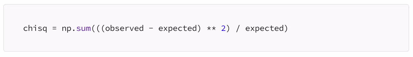
This gives us 4.23 and we also know that this statistic follows a chi-2 distribution. This is all we need to verify our null hypothesis.

Verifying the hypothesis

Let’s plot the theoretical chi-2 distribution our test statistic follows. It’s a chi-2 with one degree of freedom. The red line indicates the observed values of the test statistic.

The blue-shaded area shows the distribution the test statistic is known to follow under the null hypothesis, that is in the absence of data drift. We have just observed the value marked with the red line. Is this observation strong enough evidence to reject the null hypothesis?

A chi-2 value of, say, 10, would have been very, very unlikely to see under the null. If we saw it, we would probably conclude that the null hypothesis must be false and the data have drifted.

If we got a chi-2 value of 0.5, on the other hand, we would argue that this observed value is not really surprising under the null hypothesis, or in other words, the differences in device frequencies between training and serving data could have been produced by chance alone. In general, this means no grounds to reject the null.

But we got 4.23. How do we decide whether to reject the null hypothesis or not?

p-value

Enters the infamous p-value. It’s a number that answers the question: what’s the probability of observing the chi-2 value we got or an even more extreme one, given that the null hypothesis is true? Or, using some notation, the p-value represents the probability of observing the data assuming the null hypothesis is true: P(data|H₀) (To be precise, the p-value is defined as P(test_static(data) > T | H₀), where T is the chosen threshold for the test statistic).

Notice how this is different from what we are actually interested in, which is the probability that our hypothesis is true given the data we have observed: P(H₀|data).

what p-value represents: P(data|H₀)what we usually want: P(H₀|data)

Graphically speaking, the p-value is the sum of the blue probability density to the right of the red line. The easiest way to compute it is to calculate one minus the cumulative distribution at the observed value, that is one minus the probability mass on the left side.

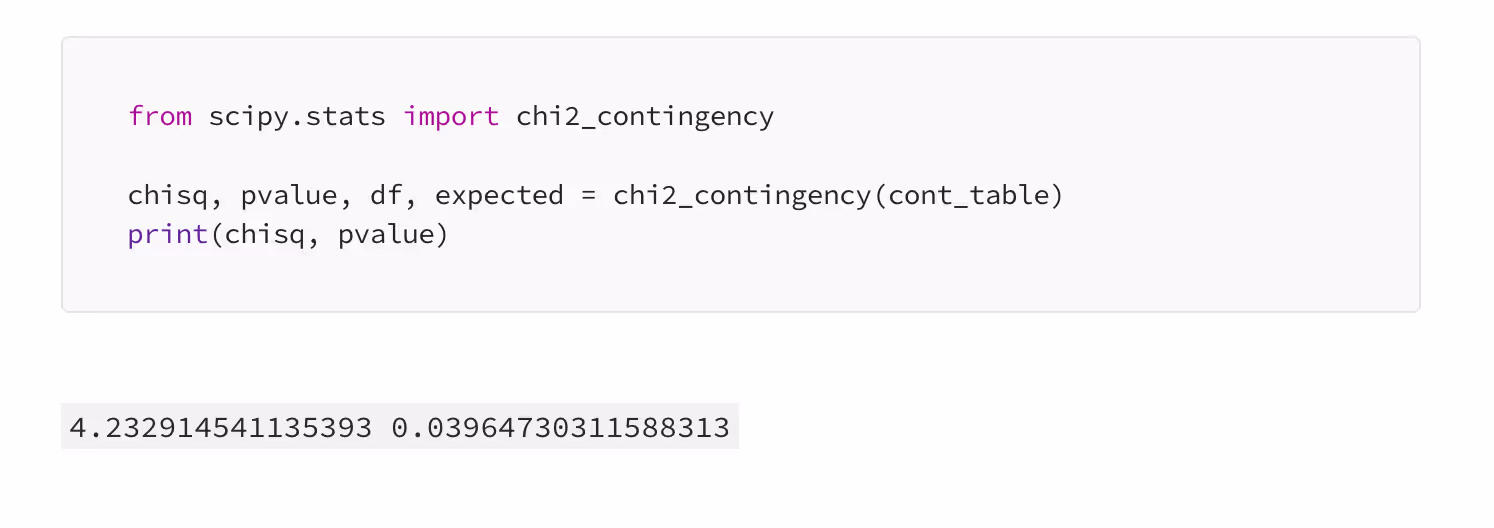
This gives us 0.0396. If there was no data drift, we would get the test statistic we’ve got or an even larger one in roughly 4% of the cases. Not that seldom, after all. In most use cases, the p-value is conventionally compared to the significance level of 1% or 5%. If it’s lower than that, one rejects the null. Let’s be conservative and follow the 1% significance threshold. In our case with a p-value of almost 4%, there is not enough evidence to reject it. Hence, no data drift was detected.

To ensure that our test was correct, let’s confirm it with scipy’s built-in test function.

This is how hypothesis testing works. But how relevant is it for data drift detection in a production machine learning system?‍

Statistical Significance vs. Monitoring Significance

Statistics, in its broadest sense, is the science of making inferences about entire populations based on small samples. When the famous t-test was first published at the beginning of the 20th century, all calculations were made with pen and paper. Even today, students in STATS101 courses will learn that a “large sample” starts from 30 observations.

Back in the days when data was hard to collect and store, and manual calculations were tedious, statistically rigorous tests were a great way to answer questions about the broader populations. Nowadays, however, with often abundant data, many tests diminish in usefulness.

The characteristic is that many statistical tests treat the amount of data as evidence. With less data, the observed effect is more prone to random variation due to sampling error, and with a lot of data, its variance decreases. Consequently, the exact same observed effect is stronger evidence against the null hypothesis with more data than with less.

To illustrate this phenomenon, consider comparing two companies, A and B, in terms of the gender ratio among their employees. Let’s imagine two scenarios. First, let’s take random samples of 10 employees from each company. At company A, 6 out of 10 are women while at company B, 4 out of 10 are women. Second, let’s increase our sample size to 1000. At company A, 600 out of 1000 are women, and at B, it’s 400. In both scenarios, the gender ratios were the same. However, more data seems to offer stronger evidence for the fact that company A employs proportionally more women than company A, doesn’t it?

This phenomenon often manifests in hypothesis testing with large data samples. The more data, the lower the p-value, and so the more likely we are to reject the null hypothesis and declare the detection of some kind of statistical effect, such as data drift.

Let’s see whether this holds for our chi-2 test for the difference in frequencies of a categorical variable. In the original example, the serving set was roughly ten times smaller than the training set. Let’s multiply the frequencies in the serving set by a set of scaling factors between 1/100 and 10 and calculate the chi-2 statistic and the test’s p-value each time. Notice that multiplying all frequencies in the serving set by the same constant does not impact their distribution: the only thing we are changing is the size of one of the sets.

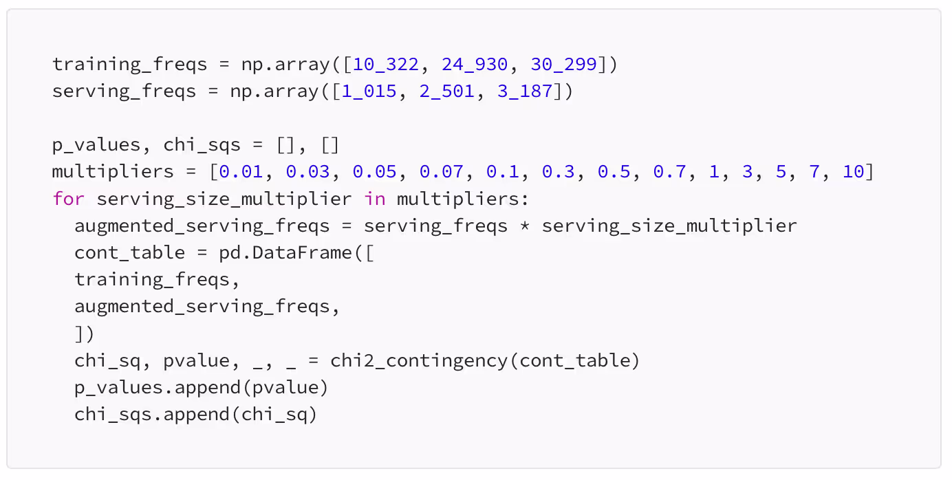
The values at the multiplier equal to one are the ones we’ve calculated before. Notice how with a serving size just 3 times larger (marked with a vertical dashed line) our conclusion changes completely: we get the chi-2 statistic of 11 and the p-value of almost zero, which in our case corresponds to indicating data drift.

The consequence of this is the increasing amount of false alarms. Even though these effects will be statistically significant, they will not necessarily be significant from the performance monitoring point of view. With a large enough data set, even the tiniest of data drifts will be indicated even if it is so weak that it doesn’t deteriorate the model’s performance.

Having learned this, you might be tempted to suggest dividing the serving data into a number of chunks and running multiple tests with smaller data sets. Unfortunately, this is not a good idea either. To understand why, we need to deeply understand what the p-value really means.

The meaning of p

We have already defined the p-value as the probability of observing the test statistic at least as unlikely as the one we have actually observed, given that the null hypothesis is true. Let’s try to unpack this mouthful.

The null hypothesis means no effect, in our case: no data drift. This means that whatever differences there are between the training and serving data, they have emerged as a consequence of random sampling. The p-value can therefore be seen as the probability of getting the differences we got, given that they only come from randomness.

Hence, our p-value of roughly 0.1 means that in the complete absence of data drift, 10% of tests will erroneously signal data drift due to random chance. This stays consistent with the notation for what the p-value represents which we introduced earlier: P(data|H₀). If this probability is 0.1, then given that H₀ is true (no drift), we have a 10% chance of observing the data at least as different as what we observed (according to the test statistic)

This is the reason why running more tests on smaller data samples is not a good idea: if instead of testing the serving data from the entire day each day, we would split it into 10 chunks and run 10 tests each day, we would end up with one false alarm every day, on average! This may lead to the so-called alert fatigue, a situation in which you are bombarded by alerts to the extent that you stop paying attention to them. And when data drift really does happen, you might miss it.

Bayes to the rescue

We have seen that detecting data drift based on a test’s p-value can be unreliable, leading to many false alarms. How can we do better? One solution is to go 180 degrees and resort to Bayesian testing, which allows us to directly estimate what we need, P(H₀|data), rather than the p-value, P(data|H₀).

What is Bayes

Bayesian statistics is a different approach to making inferences compared to traditional, classical statistics. While the founding assumptions of Bayesian methods deserve separate treatment, for the sake of our discussion on data drift, let’s consider the most important feature of the Bayesian approach: statistical parameters are random variables.

Parameters are random variables

A parameter is an unknown value that we are interested in that describes a population. In our earlier example, the proportion of our model’s users using a mobile device is a parameter. If we knew what it amounts to within any given time frame, we would be able to confidently state whether the device variable drifts over time. Unfortunately, we don’t know the devices of all possible users who might end up as the model’s inputs; we have to work with a sample of serving data that the model has received.

The classical approach regards our parameter of interest as a fixed value. We don’t know it, but it exists. Based on sample data, we can try to estimate it as well as possible but any such estimate will have some variance caused by the sampling bias. In a nutshell, we are trying to estimate what we consider to be an unknown fixed value with a random variable that has some bias and variance.

The Bayesian approach regards our parameter of interest as a random variable described by some probability distribution. What we are trying to estimate are the parameters of this distribution. Once we do this, we are entitled to make probabilistic statements about the parameter, such as “the probability that the proportion of our model’s users using mobile devices is between 0.2 and 0.6 is 55%”, for instance.

This approach is perfect for data drift detection: instead of relying on murky p-values, P(data|H₀), with a Bayesian test, we can directly calculate the probability and magnitude of data drift, P(H₀|data)!

Bayesian test for data drift

Let’s try to test whether the frequency of users using a mobile device has drifted between our training and serving data using a Bayesian approach.

Getting the probability we need

So, how does one get the probability of the data drift? It can be done using the so-called Bayes rule, a neat probability axiom allowing us to calculate the probability of something conditioned on something else if we know the reverse relation. For example, if we know what P(B|A) is, we can compute P(A|B) as:

We can use this formula to estimate the probability distribution of the frequency of mobile users, freq:

In the Bayesian jargon, all elements in the above equation have their names:

P(freq|data) is what we are after — the posterior, or the probability distribution of the mobile users' fraction after having seen the data;

P(data|freq) is the likelihood or the probability of observing the data given a particular mobile users frequency;

P(freq) is the prior: what we believe about the proportion of mobile users before seeing any data;

P(data) can be considered a scaling factor that ensures the right-hand-side sums up to one as a probability distribution should.

If we apply the above formula twice, once for the training data and then for the serving data, we will obtain two distributions for the frequency parameter: one based on the analysis data and the other based on the reference data. We can then check how the two distributions compare the test our hypothesis:

So, in order to compute the posterior, we need to multiply the prior with the likelihood and scale them to sum up to one. Arithmetics on probability distributions is not a trivial task. How do we go about it?

In some specific cases, when the two distributions match nicely, their formulas cancel out and the output of their multiplication is a known distribution. In more complex cases, Markov Chain Monte Carlo simulation methods are used to sample the values from the posterior rather than try to compute its distributional form. There is also a third way: in simple cases like ours, we can use a method called grid approximation.

Data drift probability

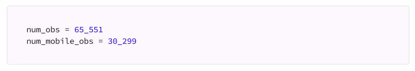
Let’s start with defining our data. In the training data, we have 65 551 observations, 30 299 of which are mobile users.

The parameter we are interested in is the frequency of mobile users. In theory, it could be any value between 0% and 100%. We will approximate it on a grid from 0.0001 to 1:

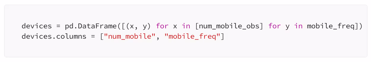
We can now create a grid of all combinations of the mobile users' frequency and their observed number:

It’s time to define a prior: what do we know or assume about our parameter before seeing any data. It could be, that we know nothing, or we don’t want to impact the results too much with our beliefs. In this case, we would adopt an uninformative prior, such as a uniform distribution. This corresponds to setting the prior to all ones, expressing the same prior probability for each possible percentage of mobile users.

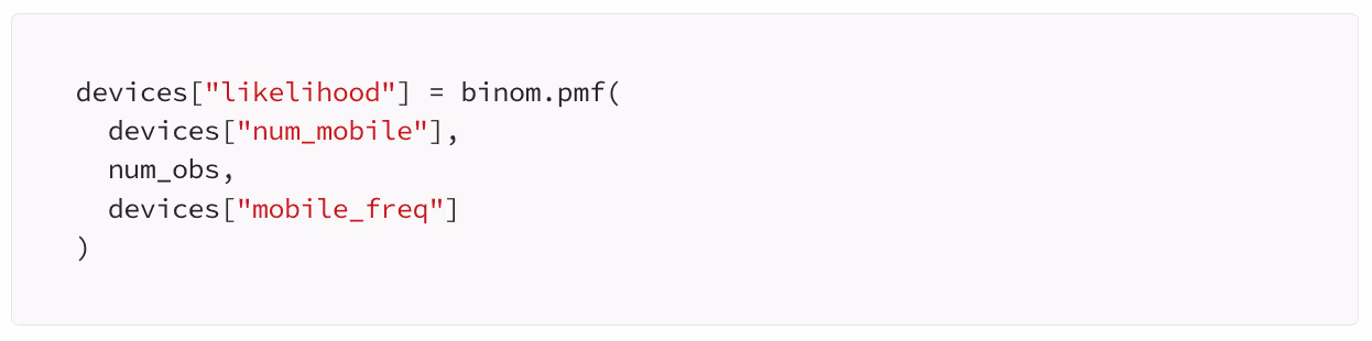
Next, our last building block, the likelihood. In our problem statement, a user can either be a mobile user or not. This calls for binomial distribution. For each row in our data frame, we will compute the likelihood as the binomial probability mass for a given number of observed mobile users, the total users, and the assumed frequency of mobile users.

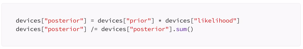
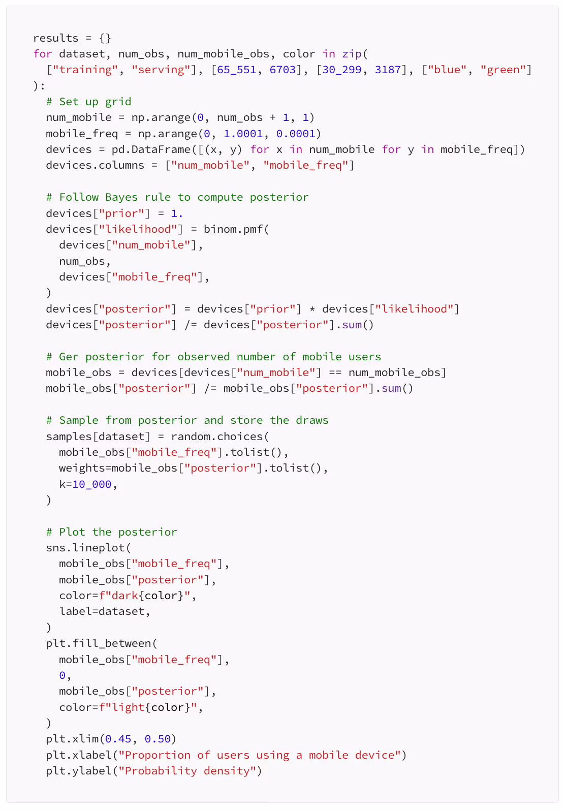
All we are left with is to follow the Bayes formula: we multiply the prior with the likelihood and scale the result to sum up to one to get the posterior.

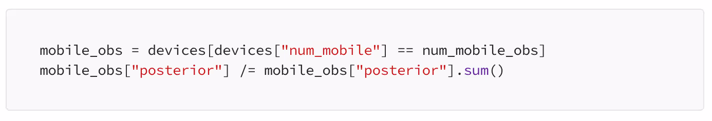
Let’s slice the grid to select the posterior that matches the number of mobile users we have observed.

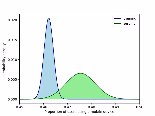
We can now plot the posterior probability of the frequency of mobile users for the training data.

We can now do the exact same thing for our serving data. While we are at it, we will add one more thing to the code: in a dictionary called samples, we will store draws from the posterior distributions, both training and serving. Here is a code snipped that does the job.

Test time

For both training and serving data, we have estimated the probability distributions for the proportion of mobile users. Is this proportion different? If so, we have some data drift going on. It seems it is different since the two distributions overlap just a little in the plot above. Nevertheless, let’s try to get a quantitative confirmation.

We can do it using the draws we have taken from both distributions: we can just check how often the serving data’s proportion is larger than the one from training data. This is our estimate of the probability of data drift.

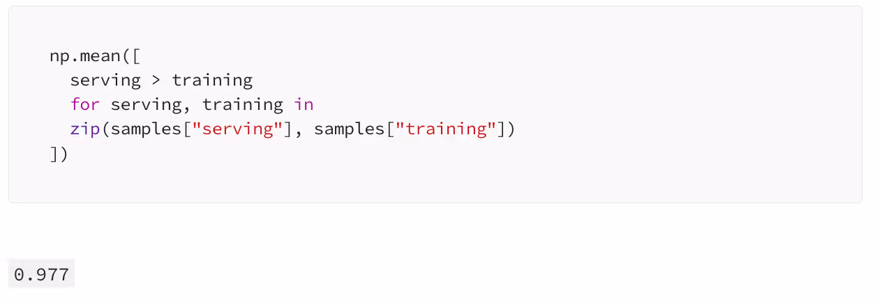
The probability that the device variable has drifted is 97.7%. The drift has almost certainly happened! But how large is it?

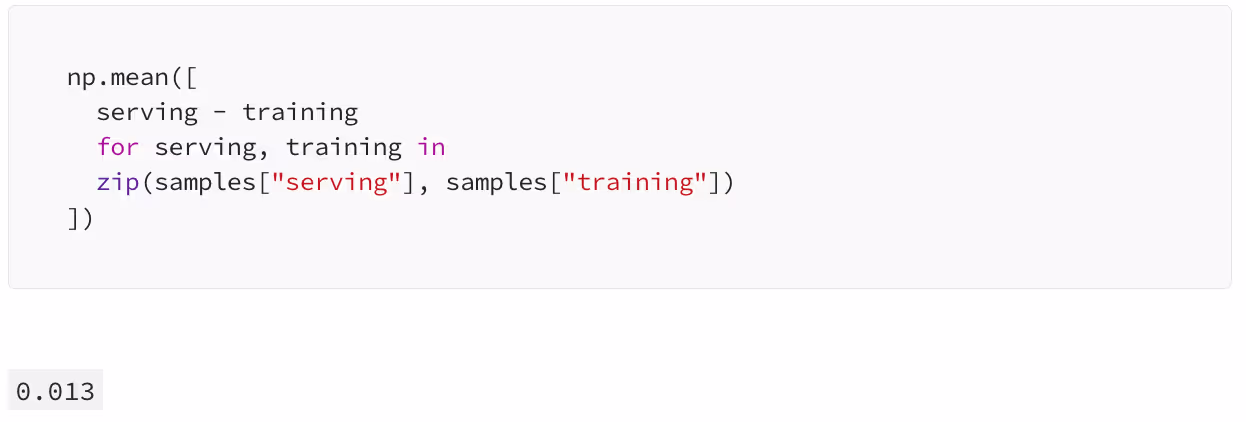
The proportion of mobile users in the serving data is larger by 1.3 percentage points than the corresponding proportion in training data, in expectation

Takeaways

Univariate data drift detection methods relying on hypothesis testing are not always reliable: the outcome might depend on the sample size and the p-value does not actually measure data drift probability or magnitude directly. Relying on such hypothesis tests tends to lead to many false alarms and alert fatigue. An alternative approach is to use Bayesian methods, which allow us to directly estimate the probability and magnitude of data drift without many drawbacks of classical testing.

If you want to learn more about univariate drift detection using NannyML, check out our docs!

We are fully open-source, so don't forget to star us on Github! ⭐

How to detect data drift with hypothesis testing