

One of the key things we look for when we monitor Machine Learning models is the existence of population shifts. Population shift means that the characteristics of the population our model is acting on have changed. We call this ‘data drift’, and for continuous variables the starting point for identifying data drift is the Kolmogorov–Smirnov test.
From theory, we know that the Kolmogorov–Smirnov test is a non-parametric test for comparing two samples. It is sensitive to both the shape as well as the locations of the distributions of the two samples. The K-S test checks whether the null hypothesis (which is that the two samples come from the same distribution) is true, and it also tells us how different the two samples are. Hence, running the K-S test gives us two values: A p-value showing us the chance of getting the two samples, assuming the null hypothesis is true, and the d-statistic showing how different the two samples are.
Understanding D-Statistic
Now we know the theory but what does that actually mean in practice?
As we said, the p-value represents the probability that we obtain the resulting samples, assuming they come from the same distribution. Assuming we aim for a 95% confidence in our conclusions, a standard practice, we require a p-value lower than 0.05 in order to discard the null hypothesis.
But what about the d-statistic? We need more intuition in order to understand what a specific value of the d-statistic means. We’ll perform some experimentation in order to do that. The key question here is how different two distributions need to be in order to generate a given number of a d-statistic? To better understand this, we’ll perform a simple experiment.
We’ll use two normal distributions, one centered around 0 with standard deviation 1, and one centered around κ with standard deviation 1. As you can see, the second normal distribution is only slightly shifted from the first. As a visual, it looks like this:

Because we can control the shift, it allows us to visualize the corresponding d-statistic. Hence, we can see the relationship between how much we need to shift a normal distribution in order to obtain a given number of the d-statistic. In order to achieve reliable results, we use samples of 20,000 points as well as 5 repeated experiments with a given number κ of shifted normal distribution, and average the results. After we run our experiments, we are able to determine the following relationship between the distance of the means of the normal distributions and the corresponding d-statistic.
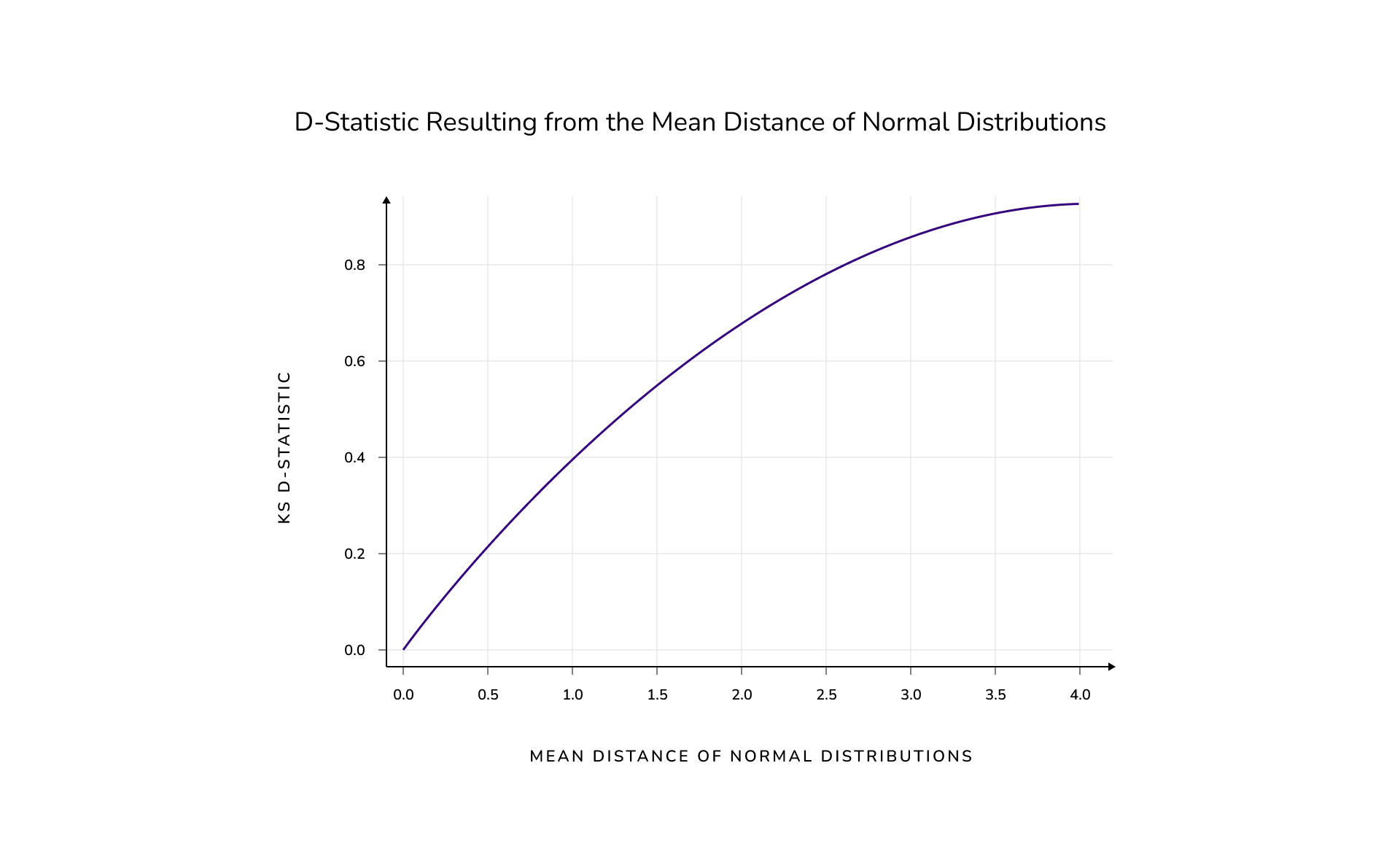
As an added tip we can also fit our results to a polynomial, and create a reference function that describes the observed relationship. We see that up to a distance of 1, between the means of the distributions, the relationship is nearly linear. As the distance grows the d-statistic tends asymptotically to one.
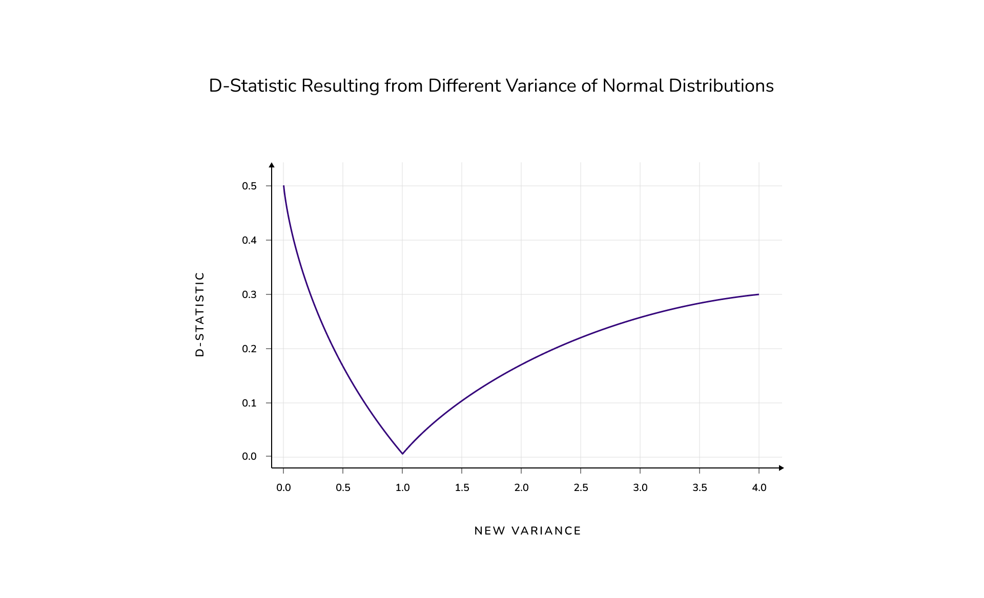
There are many ways a distribution can change, so before we continue we will explore another one. Instead of moving the mean of the second distribution, we will instead change the standard deviation of the second distribution. In this case let’s call it lambda (λ), and observe the impact on the resulting d-statistic. Our methodology is the same as the one we used previously and our results are as follows:
Now we have a better understanding of how different two distributions must be with regard to a given number of d-statistic. But how reliable are our results in practice?
Exploring Reliability
When we ask about the reliability of the results we are not speaking from a formal or theoretical perspective. We know they are solid from that respect. Instead, we are speaking from the aspect of utilizing them in production in order to make a correct assessment of data drift while monitoring data.
We will perform experiments where we introduce a known amount of drift for various sample sizes. In turn, we can then see how often our results coincide with the corresponding drift at the process which generated the data. For our new setup we‘ll use a reference sample and two “production” samples, one with drift and one without drift. We will run the K-S test on those two samples against the reference sample. The first sample will be from the same distribution as the reference sample; normal with mean 0 and standard deviation 1. The second sample will have it’s mean shifted by κ. For a successful detection we want the K-S test to not detect a significant difference for the first sample, meaning a p-value higher than 0.05. For the second sample, we want not only to detect a significant difference but also have the measure of that difference, the d-statistic, be close to the actual value. We know the actual value of the d-statistic because of the work we did on the first experiment. How close we want the d-statistic to be depends on the context of the decision we will make from that information. In this article we require the d-statistic be within a 10% range of the actual value from the process that generated the data.
One may ask, why do we test with such a strict definition of success? This is deliberate. We want to test and be sure we can rely on the K-S test for strict thresholds and resource intensive remediation actions based on them.
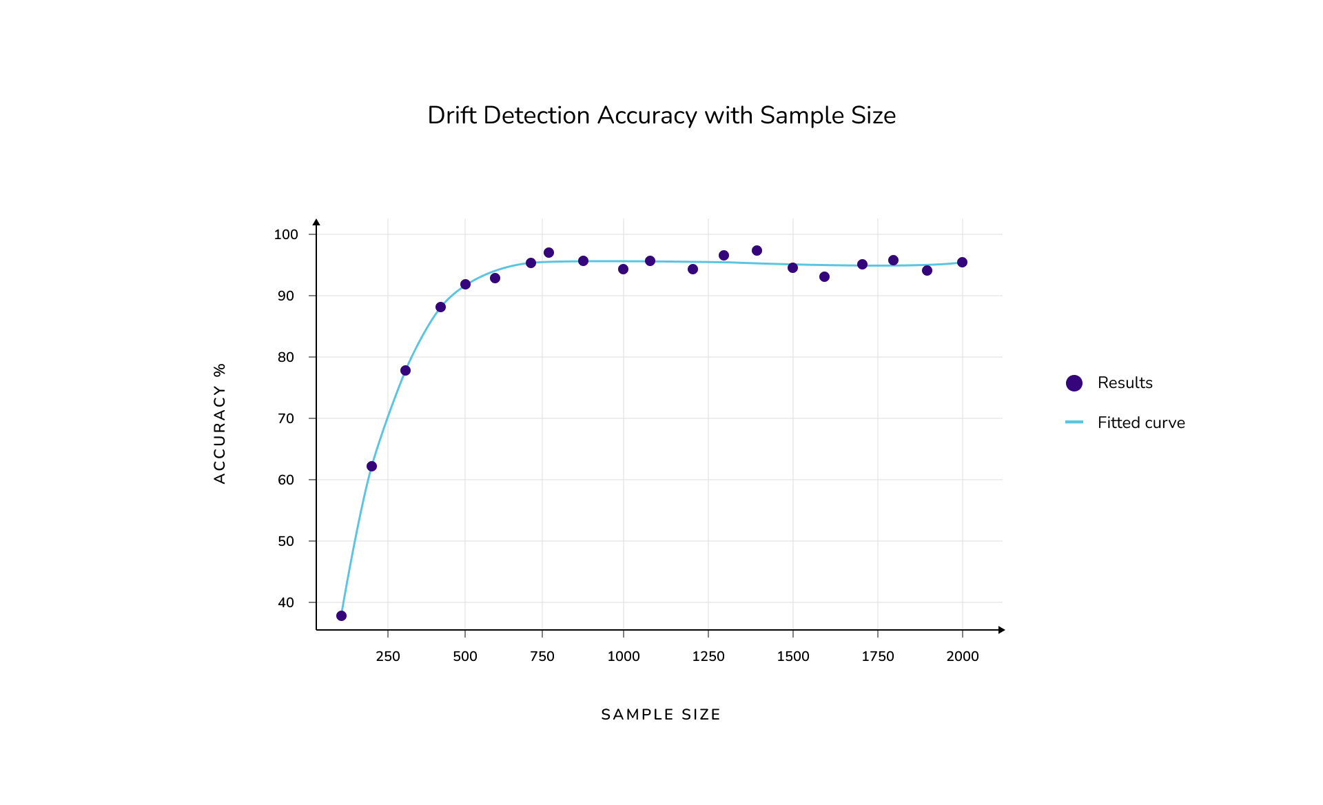
We start with a shifted mean of 0.2, 10,000 points for the reference sample, and vary the size of the production sample. We run the experiment described above 100 times and measure the ratio of successful detections as an indicator of accuracy. Below we see the influence of the production sample size on accuracy:
After looking at the results of our experiments one may wonder how many data points does a sample need to yield reliable results? To answer this question we perform our last experiment. We varied the distance of the means and used the same sample size for both reference and production samples while we searched for our target accuracy of 75%. We only looked up to a sample size of 20,000 data points to save on computation time, which is represented with the orange threshold in the plot below. We have however fitted a polynomial curve from our data to extrapolate samples sizes required to detect smaller drifts given our reliability requirement. Our results can be seen in the following graph:
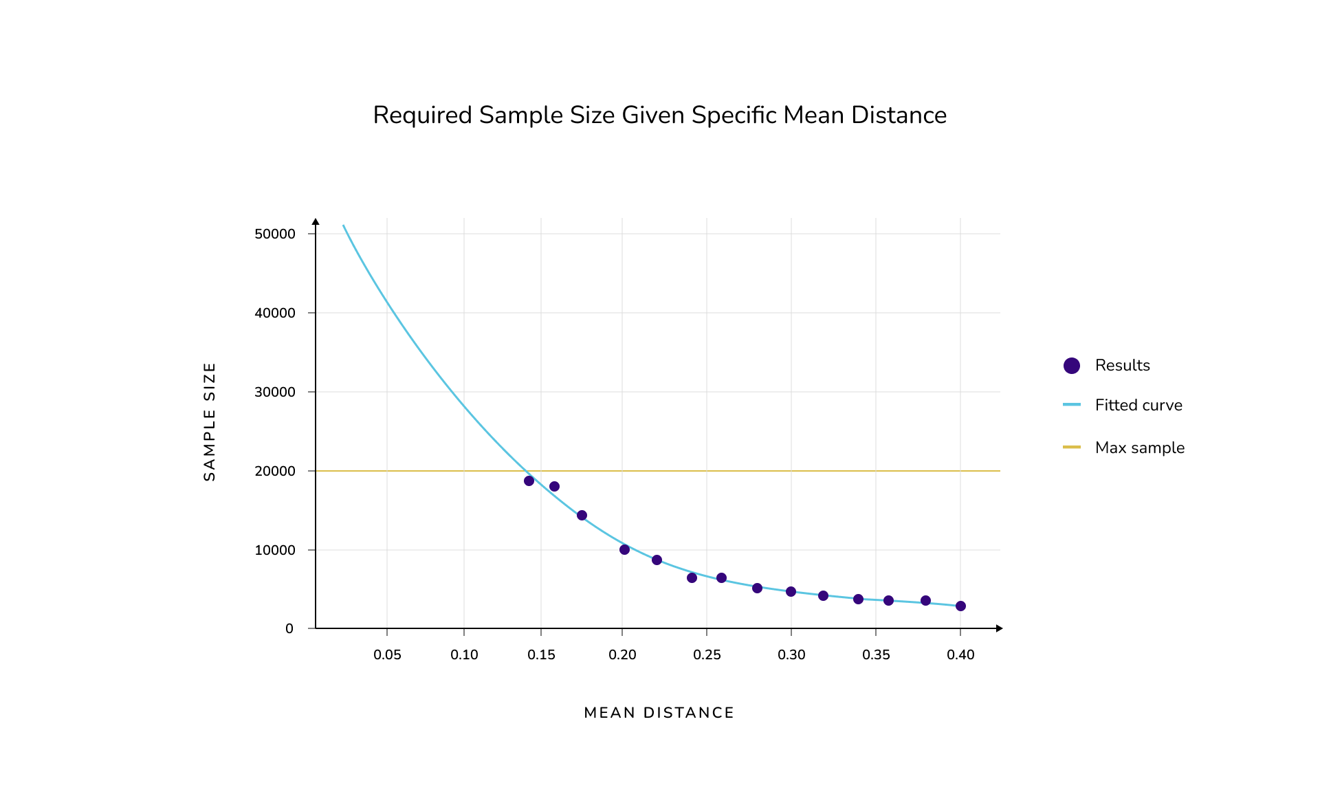
It is interesting to note that when the reference sample is the same size as the production samples, which can often happen in production, relatively large sample sizes are needed in order to establish reliable drift detection.
Conclusion
Starting from the solid theoretical foundations of the K-S test, we explored how close they are to the “ground truth”. This refers to the actual processes where our data originates, describing situations that could happen in a production setting. The key takeaway is that because of the random variance inherent in those settings, we need to take care when relying on the K-S test to make decisions. Simply put, due to the statistical nature of the problem, the results of the test may not be as accurate as we think. It may well be more appropriate that we change the parameters of the test to achieve more reliable results, for example by increasing the sample size, or use additional context to inform our decisions.


.avif)