The growing number of Machine Learning (ML) models deployed to production caused i.i.d.^* to become another example of wishful thinking. The World is changing. Data is changing. ML models stay the same though. They don’t adapt automatically (yet). To make the right decision on when and how to adapt the model, you need to monitor the changes in data that affect your model.

In this series of three articles, we will explore the main types of data change (data drift), their effect on target distribution, and model performance. We share findings that we have learned and developed while researching data drift detection and performance estimation methods at NannyML. So, if you haven’t heard about covariate shift, concept shift, and label shift - you’re in good hands. If you have read about them many times already – that’s even better, I bet you will find this interesting.

This article is part of a series of three, where we'll discuss about covariate shift, concept shift and label shift.

The concepts and ideas in this article are described with binary classification in mind. We will often refer to an example of credit default prediction. This simplifies the description and helps to build the intuition. When well-understood, these concepts can be generalized to other tasks.

^*i.i.d - the assumption that input data is an independent and identically distributed collection of random variables.

‍

Data drift

Data drift is any change in the joint probability distribution of input variables and targets (denoted as $P(X,Y)$) ^[1]. This simple definition hides a lot of complexity behind it.

Notice the keyword joint. Data drift can take place even if none of the individual variables drifts in separation. It might be the relationship between variables that changes.

There are different types of data drift, depending on the type of change that happens in this joint probability distribution and a causal relationship between inputs and targets.

The two most popular ones mentioned in almost every data-drift-related piece of content are covariate shift and concept shift. Even if you have already read about them tens of times, read again. This time it is going to be different. Trust me.

‍

Covariate shift

What it really is

Covariate is just another name for model input variable (or feature).

Pure covariate shift is then a change in the joint probability distribution of input variables provided that conditional probability of target given inputs remains the same ^[1].

Putting it simpler– it is a change in the inputs distribution with the relationship (not necessarily causal) between inputs and target remaining unchanged.

An example of covariate shift in credit default use case would be an increase in the fraction of applicants with low income with the relationship between income and probability of default remaining unchanged.

The product rule

This is a good place to introduce a widely used equation of the probability product rule:

$P(Y,X) = P(Y|X)P(X)$

This time we will actually explain it and make use of it. Don’t worry, there won’t be a lot of heavy math or statistics, just the basics.

Let’s start from the $P(Y|X)$ term – this is a conditional probability of targets given inputs. It represents the true probabilistic relationship between inputs and targets. We call it concept. This is what ML models learn based on data.

‍For example: a trained sklearn classifier holds a representation of the learned concept which maps inputs to expected target probabilities through the predict_proba method. In general, it can be represented as the distribution of targets given distribution of inputs. In case of binary classification, $P(Y|X)$ can be imagined as two hyper surfaces over the whole input space. This is tricky. Let’s build our intuition from the bottom up.

While keeping in mind the credit default use case consider only a single observation – a single credit applicant described with a set of $m$ input features:

$X=(x_1,x_2,…,x_m)$

Let’s also focus on single target value: $Y=1$. Now the concept term becomes:

$P(Y=1│X=x_1,x_2,…,x_m )$

and it represents the probability of defaulting for a specific set of inputs (an applicant). It is a single number, a scalar, for example $0.2$. Let’s simplify even further and imagine our model has only one input feature, so $X$ is 1d. We now have $P(Y=1|X=x_1)$ which is still a scalar. $P(Y=1|X)$ however is now a curve – it expresses the probability of default for all possible values of x. We can easily imagine and plot it:

For a second let’s forget about inputs distribution and focus on target alone i.e. on $P(Y)$. Let’s drop the $Y=1$ simplification for a while. For binary classification, target can take two values: $0$ or $1$. The probability of seeing one value defines the probability of seeing the other – if we have 20% probability of observing $1$ then it means we have 80% probability of observing $0$. Now, for a selected observation, the probability of targets given input becomes a pair of scalars:

$P(Y│X=x_1,x_2,… x_n)= (0.8,0.2)$

For 1d input $P(Y|X)$ are two curves over the range of $x$, for 2d – two surfaces over the area created by $x_1$ and $x_2$ and for 3 and more - $P(Y|X)$ are two hypersurfaces over the whole input space.

I hope it became clear now. In the rest of the text we will stick to $Y=1$ assumption most of the times as it simplifies things without losing any information.

Now the other term - $P(X)$.

This, I think, is simpler – it is just a joint multivariate probability distribution of all input variables/features. If an input is a categorical (discrete) variable it is a probability of each category or probability mass function (PMF). For continuous input we can simplify and imagine this as probability density function (PDF) although this is not strictly correct^*. We can visualize both:

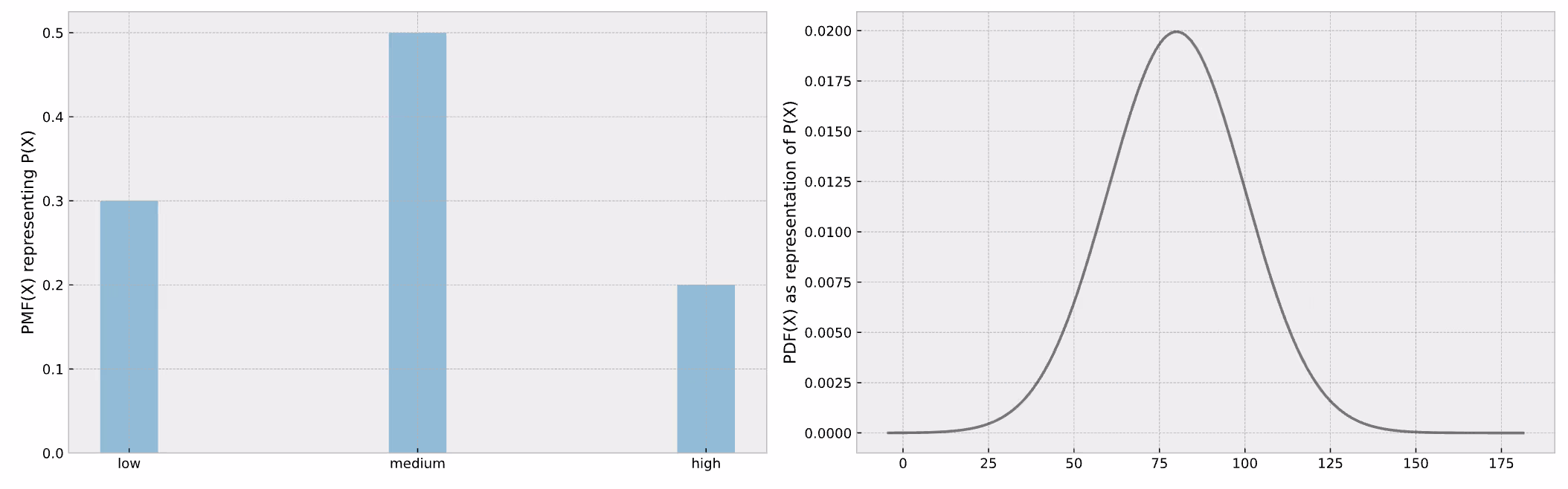
^*For PMF probability of seeing a specific discrete value is defined so $PMF(x=x_1)=P(X=x_1)$ which is a scalar. For continuous variable the notion of probability exists only in the ranges of $X$ so $P(x_1<X<x_1+dx)$ is an integral of $PDF(X)$ in the range from $x_1$ to $x_1+dx$.

The magnitude of covariate shift

We have the basics sorted, let’s go back to covariate shift. In pure covariate shift the concept $P(Y|X)$ remains the same while the probability distribution of inputs $P(X)$ changes. This causes a change of $P(Y,X)$ which – as we already mentioned – is the joint probability distribution of inputs and targets.

Let’s talk examples.

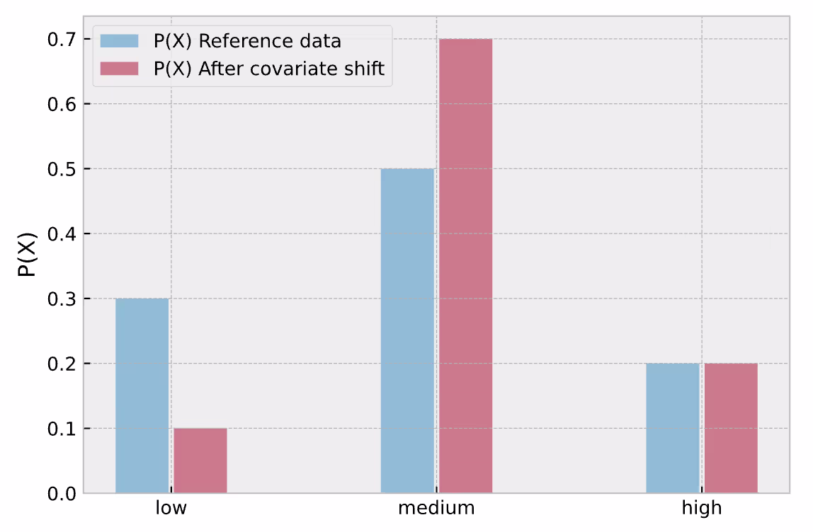
Assume again that our credit default model has only one input variable – income. Consider it a categorical variable with three categories – low, medium, high. In the training data of our model we have:

• 30% low,
• 50% medium,
• 20% high-income applicants.

Now imagine that economy is getting better and there are less low-income applicants. We now have:

• 10% low,
• 70% medium,
• 20% high-income applicants.

This can be visualized:

The first natural question to ask is – how to express the magnitude of covariate shift? An intuitive and easily interpretable measure is a sum of absolute differences of $P(X)$ for each of $i$ classes:

$\dfrac{1}{2}\sum_{i} \bigg|P(X=x_i )_{shifted} -P(X=x_i )_{reference}\bigg|$

or in general case – the absolute difference between input distributions:

$\dfrac{1}{2}\sum_{X} \bigg|P(X)_{shifted} -P(X)_{reference}\bigg|$

The difference is multiplied by $ \frac{1}{2}$ to avoid measuring the same change twice (if one of the categories dropped by $0.1$, other categories had to increase by $0.1$ – if we count both, the total change will be $0.2$ but the intuition says that the actual change is $0.1$). As a side effect, the result falls into $0 - 1$ range - $0$ means that nothing has changed while $1$ means there is no overlap at all between reference and shifted data. In our case that would be:

$ \dfrac{1}{2} (|0.1-0.3|+|0.7-0.5|+|0.2-0.2|)=0.2$

This indeed is interpretable, especially in simple cases like the example analyzed, as exactly 20% of applicants has moved from one category to the other.

The effect of covariate shift on target distribution

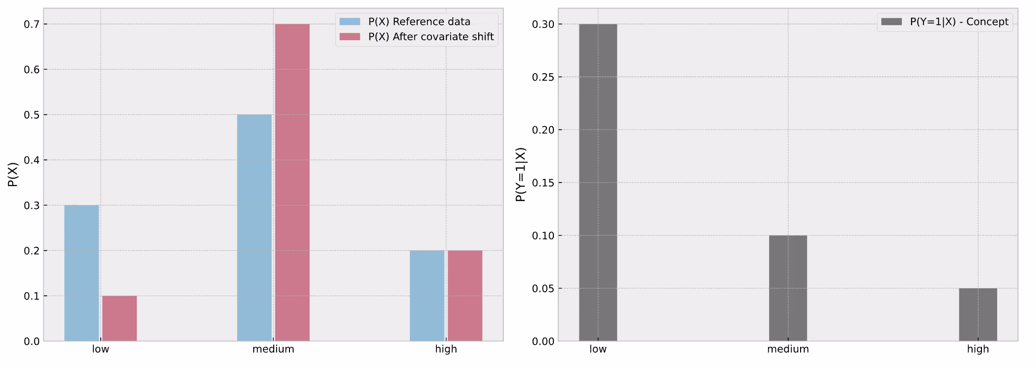
We know the magnitude of covariate shift already. Now we are interested to see what is the impact on target distribution. We need concept for this. Let’s assume conditional probabilities of default given income for each income category:

• $P(Y=1|X=low\;income) =0.3$,
• $P(Y=1|X=medium\;income) = 0.1$,
• $P(Y=1|X=high\;income) = 0.05$.

Showing the full story in single plot now:

Let’s forget about covariate shift for a second and look at the reference period only. What is the overall probability of seeing an event of low-income applicant defaulting? Product rule to the rescue.

It is $P(Y=1|X=low\;income)$ multiplied by $P(X=low\;income) = 0.3\cdot0.3 = 0.09$. It means that in reference data we observe 9% of low-income clients defaulting. For medium and high-income applicants this is respectively 5% and 1%. That is our initial target distribution with respect to input. Now, after covariate shift this becomes:

• $0.3\cdot0.1 = 0.03$ for low,
• $0.1\cdot0.7 = 0.07$ for medium,
• $0.05\cdot0.2 = 0.01$ for high-income.

So until now we have applied product rule to reference input distribution and shifted input distribution while keeping the concept the same:

$P(Y,X)_ {reference}=P(Y|X)_{reference} P(X)_{reference}$

$P(Y,X)_ {shifted}=P(Y|X)_{shifted} P(X)_{shifted}$

Now we can compare these two and summarize changes in categories:

• a drop from 0.09 to 0.03 in low-income group,
• an increase from 0.05 to 0.07 in medium-income,
• no change in the high-income group.

Plotting again:

These differences calculated can be used as the measure of covariate shift effect on target distribution. An absolute magnitude of this effect for binary classification is:

$\sum_{X} P(Y=1|X)_{reference}\cdot\bigg|P(X)_{shifted}-P(X)_ {reference}\bigg|$

Or:

$\dfrac{1}{2}\sum_{X} P(Y|X)_{reference}\cdot\bigg|P(X)_{shifted}-P(X)_ {reference}\bigg|$

For our example this is:

$0.3\cdot|0.1-0.3|+0.1\cdot|0.7-0.5|+0.05\cdot|0.2-0.2|=0.08$

The interpretation is that 8% of targets have changed its expected value due to covariate shift, either from $0$ to $1$ or from $1$ to $0$.We can also calculate the directional change (non-absolute):

$\sum_{X} P(Y=1|X)_{reference}\cdot (P(X)_{shifted}-P(X)_ {reference})$

$0.3\cdot (0.1-0.3)+0.1\cdot (0.07-0.05)+0.05\cdot (0.2-0.2)=-0.04$

In binary classification the directional effect on target distribution is equal to the expected change in class balance. So in our case, due to the covariate shift we expect 4 percentage point less defaults among all the applicants.

Impact of covariate shift on performance

We already discussed the business effect of covariate shift – there are less low-income people amongst applicants and less applicants defaulting in general. Whether that’s good or bad – it depends on the business-related stuff (like business goals, dependence of profitability of credits on applicants’ income and default probability etc.) Data-science-wise we might wonder what’s the effect of covariate shift on performance of the model. Let’s have a look at the following plot:

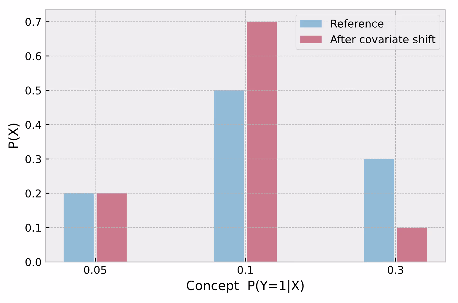
For all the considerations we assume our model is indeed probabilistic and it returns well calibrated probabilities (meaning among applicants which credit default probability was estimated to be 10%, 10% will default). With this assumption the concept that we see on x-axis is equal to the probability predicted by our model. On y-axis we see what is the proportion of specific predictions (which is equal to the proportion of inputs for which the concept maps them to the specific probability for class 1, hence $P(X)$).

We see that due to covariate shift we will predict probability of 0.1 more often compared to reference period while 0.3 prediction will be less likely. In that case the model will get better according to most of the metrics generally used for binary classification (accuracy, f1, ROC AUC etc.) Why exactly? Because we have less predictions from high-uncertainty region (close to 0.5) and more from low-uncertainty region (close to 0 and 1). Since explaining this in detail is not the purpose of this (already too long and getting longer) blog post check out more information here if you are not convinced.

Anyways, covariate shift has improved our model – that’s great, but can we just enjoy the stroke of luck and do nothing? Not really. Theoretically, when experiencing pure covariate shift, model performance cannot be improved by retraining –because the concept that is learnt by the model stayed the same. In reality, however, we just got more data from a specific region in the input space. It may turn out that this region was previously underrepresented and the concept our model learnt can be improved there. Definitely worth investigating. Another thing is that covariate shift may foreshadow concept shift happening soon^*.

We will discuss concept shift later, now we will go through the same analysis for continuous input.

^*Alright you got me – it may or may not. I wanted to introduce some drama. The gut feeling however is that when observable data changes we expect the unobservable data may change – just as in the world we live in, everything impacts everything in a sense, so if one thing changes we expect other to change as an effect, sooner or later. And the change of unobservable data that is causally related with the target is a concept shift. We will explain that later.

Same analysis for continuous input

We have a single categorical input analyzed, let’s see what happens with continuous variable.

When you write a master thesis at a technical university they tell you to take your bachelor thesis and replace all the sums with integrals and all the difference with differentials and it’s ready. It’s the case here when switching to covariate shift in continuous variables.

Imagine again our single-input model, but this time with continuous, normally distributed income. The covariate shift and the unchanged concept are as follows:

Now the magnitude of covariate shift alone becomes:

$\dfrac{1}{2}\int_X\bigg|pdf(x)_ {shifted}- pdf(x)_ {reference}\bigg|dx$

We can clearly show the integral in the plot:

The value calculated for our case is 0.38. What does it mean? Notice the 90 €k threshold where the two pdfs cross. After covariate shift there are less people in <90 €k range and more people in >90 €k range. Exactly 38% of applicants migrated from <90 €k range to >90 €k range.

Now let’s take concept into account and calculate the absolute effect of pure covariate shift on target distribution.

Denoting concept $P(Y=1|X)$ as $c(x)$ we have:

$\int_Xc(x)_ {reference}\cdot\bigg|pdf(x)_ {shifted}- pdf(x)_{reference}\bigg|dx$

The directional effect is simply:

$\int_Xc(x)_ {reference}\cdot(pdf(x)_ {shifted}- pdf(x)_{reference})dx$

The integrands can be plotted:

The absolute and directional effects have exactly the same meaning as in case of categorical variable. Let’s focus on the directional effect as it shows the full picture (right-hand side plot).

We can see that in the 0-90k €/y area the effect of covariate shift on target distribution is negative. That’s expected – as a result of the income increase there are relatively less applicants with income in that range so we will observe less people defaulting from 0-90k €/y area. On the other hand, the amount of applicants with income >90k €/year has increased and we will observe more people defaulting from that group. At the end of the day, the negative effect is stronger (red area is larger than green) because of higher concept values in the negative effect range. The fraction of applicants defaulting will drop exactly by 6.9 % (as calculated using the directional integral).

When it comes to effect of covariate shift on model performance metrics – just like in categorical case, model has improved due to covariate shift as there are relatively more predictions from lower-uncertainty regions:

‍

In this article, we introduced the notion of covariate shift, how it really works and its impact on performance metrics. In part 2 we explain the topic of concept shift following the same structure. Continue reading here

‍

Summary

Let’s recall all the measures of covariate shift that we have introduced:

1. Pure covariate shift effect that does not take concept into account. It tells how severe is the covariate shift alone,

$\dfrac{1}{2}\int_X\bigg|pdf(x)_{shifted}-pdf(x)_{reference}\bigg|dx$

‍

2. The absolute and directional effects of covariate shift on target distribution. First tells the fraction of targets affected, the second tells the direction of the change (the effect on class balance):

$\int_Xc(x)_ {reference}\cdot\bigg|pdf(x)_ {shifted}- pdf(x)_{reference}\bigg|dx$

$\int_Xc(x)_ {reference}\cdot(pdf(x)_ {shifted}- pdf(x)_{reference})dx$

‍

What’s described here is a part of the research we do at NannyML. Some of it does not come from reviewed articles so we might be wrong here and there (well, reviewed articles can be wrong as well). Let us know if you find any mistakes in our reasoning. Explore the notebook linked to check the results on your own.

‍

References

[1]: Moreno-Torres, J.G., Raeder, T., Alaíz-Rodríguez, R., Chawla, N., & Herrera, F. (2012). A unifying view on dataset shift in classification. Pattern Recognit., 45, 521-530.

Cover Image: Utaraitė, N. (2021). Here Are 18 Photos Showing Dog Breeds Today Vs. 100 Years Ago. Boredpanda. https://www.boredpanda.com/dog-breeds-100-years-ago-and-today

‍

NannyML is fully open-source, so don't forget to support us with a ⭐ on Github!

If you want to learn more about how to use NannyML in production, check out our other docs and blogs!