

In part 1 of this series, we covered the topic of covariate shift in depth, and introduced the notion of concept. Even if you came here for concept shift only, read it first.
Now it’s time to go into detail and tackle another big monster, concept shift. First, a refresher of what is data drift:
Data drift
Data drift is any change in the joint probability distribution of input variables and targets (denoted as $P(X,Y)$) [1]. This simple definition hides a lot of complexity behind it.
Notice the keyword joint. Data drift can take place even if none of the individual variables drifts in separation. It might be the relationship between variables that changes.
There are different types of data drift, depending on the type of change that happens in this joint probability distribution and a causal relationship between inputs and targets.
The two most popular ones mentioned in almost every data-drift-related piece of content are covariate shift and concept shift. Even if you have already read about them tens of times, read again. This time it is going to be different. Trust me.
Concept shift
What it really is
Concept is the relationship between covariates (features) and the target. Pure concept shift is a change in the conditional probability of inputs given targets provided that joint probability of inputs remains the same. So $P(Y|X)$ changes, $P(X)$ stays the same and $P(Y,X)$ changes as an effect[1] (due to product rule, didn’t I tell you to read about covariate shift first?).
An example of concept drift in our use case would be: fraction of low-income people applying for credit remains unchanged, but the likelihood that low-income applicant will default changes.
Bayesian view
When we view our model as a Bayesian network we can define concept shift as a shift in unobserved variables which directly or indirectly cause the target with no observed variables on causal path. Sounds complicated but it will get simple soon. Let’s imagine that the network below is true for our simple model:
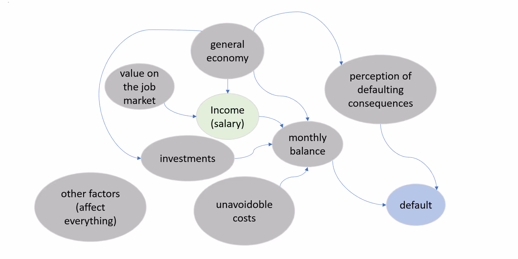
In this graph arrows indicate true causal relationships. This simplified model of reality assumes that there are two factors that directly cause clients to default – whether they can afford to pay the loan back (monthly balance) and whether they consider it beneficial to pay it back (perception of defaulting consequences).
First thing to notice is that there is no direct arrow between the income and default probability.That’s what I meant at the beginning when defining concept as the relationship between income and defaulting probability as mapping between these two that can be learned (which is not necessarily causal). Again, that’s what ML models do – they learn the mapping.
In causal world a job salary has no direct effect on probability of credit default. We can earn a lot but need to spend a lot as well. We may also not work at all but have other sources of money (like investments or savings). So income affects target through monthly balance. Income itself in this simple model is caused by general economy situation and applicant’s value on the job market.
Let’s consider following population-level shifts (i.e., shifts that are real trend for all applicants, not for a single one):
- client’s value on the job market shifts (for whatever reason, let’s not complicate this by details) – notice that there is no other path to affect the target other than the one leading through the observed income variable. What does it mean? That the change in client’s value on the job market that is relevant for the target will always be observed in the income variable. From our perspective it just looks like the income distribution has changed and the targets distribution changed accordingly – with the mapping between them remaining the same. This will be a pure covariate shift.
- unavoidable costs shift - this will affect the target through monthly balance variable and won’t be noticed by income. This shift will change the target distribution without affecting the income distribution. What happens then is that the input (income) distribution remains the same but the target distribution changes. From our (and model) perspective the mapping between income and target will have to change then as we see different targets for the same inputs. This will be a pure concept shift.
- general economy shifts – this usually will be seen as both – covariate shift and concept shift as it affects the observed variable and the target through a path that does not contain the observed variable.
I found this view on concept shift more comprehensive. An alternative is just saying that the concept is changing, for whatever reason. But this reason is always related to another change in the system which is unobserved or might be even unmeasurable. For example – buyers decisions may change due to social media influencers changing their perception of a specific behavior or a product. This perception change is unmeasurable but it has real, measurable effect of concept change.
The magnitude of concept shift
We are already familiar with the credit default model example and we will explore it further. We have some intuition already so we can take shortcuts. We will go straight to continuous input variable case as I found them more insightful.
The situation is: income distribution stays the same, concept changes:

Qualitatively we see that the concept has changed in the following way – applicants with income <93 k€/y became more likely to default while the ones earning >93 k€/y became less. The change for <93 €k/y group is stronger (the difference is larger).
Let’s quantify that. Recall that we have denoted concept $P(Y=1|X)$ as $c(x)$. The absolute magnitude of pure concept shift effect is:
$\dfrac{1}{x_{max}-x_{min}}\int_{x_{min}}^{x_{max}}\bigg|c(x)_{shifted}-c(x)_{reference}\bigg|dx$
The first term (outside of integral) is a normalization factor that ensures that the result of integration converges and is meaningful. Otherwise it would increase together with increase of the difference between integral limits $x_{min}$ and $x_{max}$.
How to define $x_{min}$ and $x_{max}$? This is a range in which $x$ exists as the concept itself exists only where data exists. Theoretically $x$ exists everywhere (ranges from $-\infty$ to $+\infty$) as pdf of normal distribution will return a positive value for any $x$. In reality this is limited and in practice this could be just minimum and maximum value of that variable seen in the data sample.
The normalization term also ensures that the value of the proposed concept shift measure is in the range $0-1$. $0$ means there is no concept shift at all. $1$ means that all the targets would change its expected value – either from $0$ to $1$ or the other way around.
This measure does not take into account the probability distribution of $x$ - it doesn't care how exactly input data is distributed, it only cares where $x$ and concept exist, which is between $x_{min}$ and $x_{max}$. Therefore it does not tell how target is affected with our specific $P(X)$. It tells how severe is the concept shift alone and how the target would be affected if it was uniformly distributed in the range between $x_{min}$ and $x_{max}$. In the analyzed case concept shift magnitude equals 0.043.
The effect of concept shift on target distribution
We have calculated the magnitude of concept shift alone, now we want to see its impact on target distribution when we include the actual probability distribution of the input. We can calculate the absolute impact with:
$\int_xpdf(x)_ {reference}\cdot\bigg|c(x)_ {shifted}- c(x)_{reference}\bigg|dx$
and the directional one:
$\int_xpdf(x)_ {reference}\cdot(c(x)_ {shifted}- c(x)_{reference})dx$
The terms inside integrals can be visualized:

Let’s look at the directional change. In the <93 k€/y region concept shift has positive effect on target distribution as the probability of default for this income range has increased. It is additionally boosted by the fact that there are generally more <93 k€/y applicants then >93 k€/y. The final effect on target distribution will be then positive and equal to about 3% - we will see an increase of defaults by 3 percentage points.
The effect of concept shift on model performance
Generally, pure concept shift will always have negative effect on model performance. Concept is what model learns and if this changes model just becomes worse. Performance drop depends on how strong the concept shift is and how much data is affected by it.
This article introduces concept shift, what it really is and its impact on performance metrics. To learn more about the interaction between covariate and concept shift check out the third part of this series. If you've missed the explanation of covariate shift go back to the first article :)
Summary
Let’s recall all the measures of concept shift that we have introduced:
1. Pure concept shift effect that does not take input distribution into account. It tells the severity of concept shift alone – what is the fraction of targets that would be affected if $x$ was uniformly distributed:
$\dfrac{1}{x_{max}-x_{min}}\int_X\bigg|c(x)_{shifted}-c(x)_{reference}\bigg|dx$
2. The absolute and directional effect of concept shift on target distribution. First tells the fraction of targets affected, the second tells the direction of the change (the effect on class balance):
$\int_Xpdf(x)_ {reference}\cdot\bigg|c(x)_ {shifted}- c(x)_{reference}\bigg|dx$
$\int_Xpdf(x)_ {reference}\cdot(c(x)_ {shifted}- c(x)_{reference})dx$
What’s described here is a part of the research we do at NannyML. Some of it does not come from reviewed articles so we might be wrong here and there (well, reviewed articles can be wrong as well). Let us know if you find any mistakes in our reasoning. Explore the notebook linked to check the results on your own.
References
[1]: Moreno-Torres, J.G., Raeder, T., Alaíz-Rodríguez, R., Chawla, N., & Herrera, F. (2012). A unifying view on dataset shift in classification. Pattern Recognit., 45, 521-530.
NannyML is fully open-source, so don't forget to support us with a ⭐ on Github!
If you want to learn more about how to use NannyML in production, check out our other docs and blogs!
Read part I of the blog series - Understanding Data Distribution Shifts in Machine Learning I: Covariate Shift
Read part III of the blog series - Understanding Data Distribution Shifts in Machine Learning III: Interaction between Covariate and Concept Shift


.avif)