Why is Machine Learning Monitoring in production hard?

Do not index

Canonical URL

Introduction

Being a data scientist may sound like a simple job - preparing data, training a model, and deploying it in production. However, the reality is far from easy. The job is more like caring for a baby - a never-ending cycle of monitoring and ensuring everything is fine.

The challenge lies in the fact that there are three key components to keep an eye on: code, data, and the model itself. Unfortunately, each element presents its difficulties, making monitoring in production hard.

In this article, we will dive deeper into those challenges and mention possible solutions.

Two ways a machine learning model can fail

The model fails to make predictions

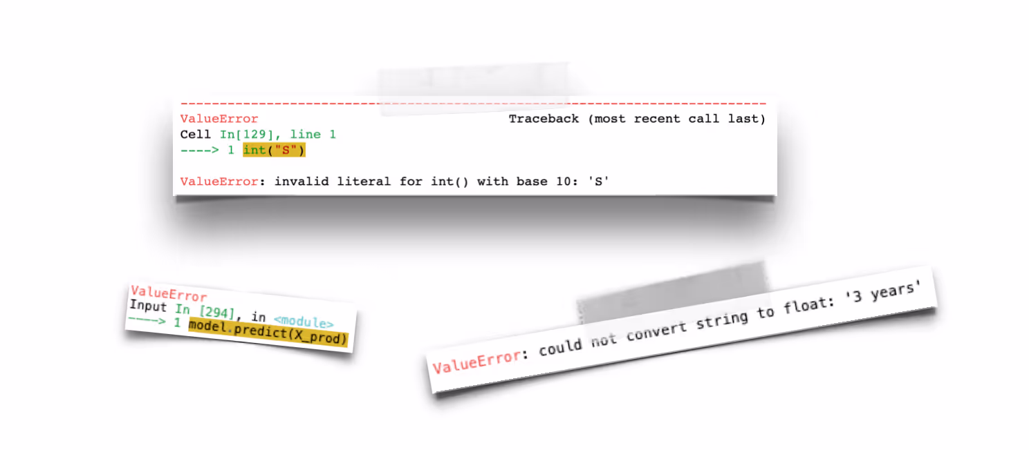
When we talk about a model failing to make a prediction, it means it cannot generate an output. Since the model is always a part of a larger software system, it's also exposed to more technical challenges. Here are a few possible examples:

Language barriers - integrating a model built in one programming language into the system written in a different one. It might require additional code or "glue" code to connect the two languages, increasing complexity and risk of failure.

Maintaining the code - as we know, libraries and other dependencies are constantly updated, so their function commands, etc. It's essential to keep track of those changes in relation to the code so it stays relevant.

Scaling issues - as our model gets more and more users, the infrastructure may need to be more robust to handle all requests.

Well-maintained software monitoring and maintenance system should prevent possible problems. However, even if something happens, we get direct information that something is wrong. In the next section, we will look into the problems in which detection is not so obvious.

The model’s prediction fails

In this case, the model generates the output, but its performance is degrading. This type of failure is particularly tricky because it is often silent - there are no obvious alerts or indicators that something is happening. As a result, the whole pipeline or application is functioning well, but the predictions produced by the model may no longer be valid.

Model performance degradation can happen for two reasons:

Covariate Shift

A model can fail to make accurate predictions in the presence of covariate shift, i.e., when the distribution of the input features changes over time.

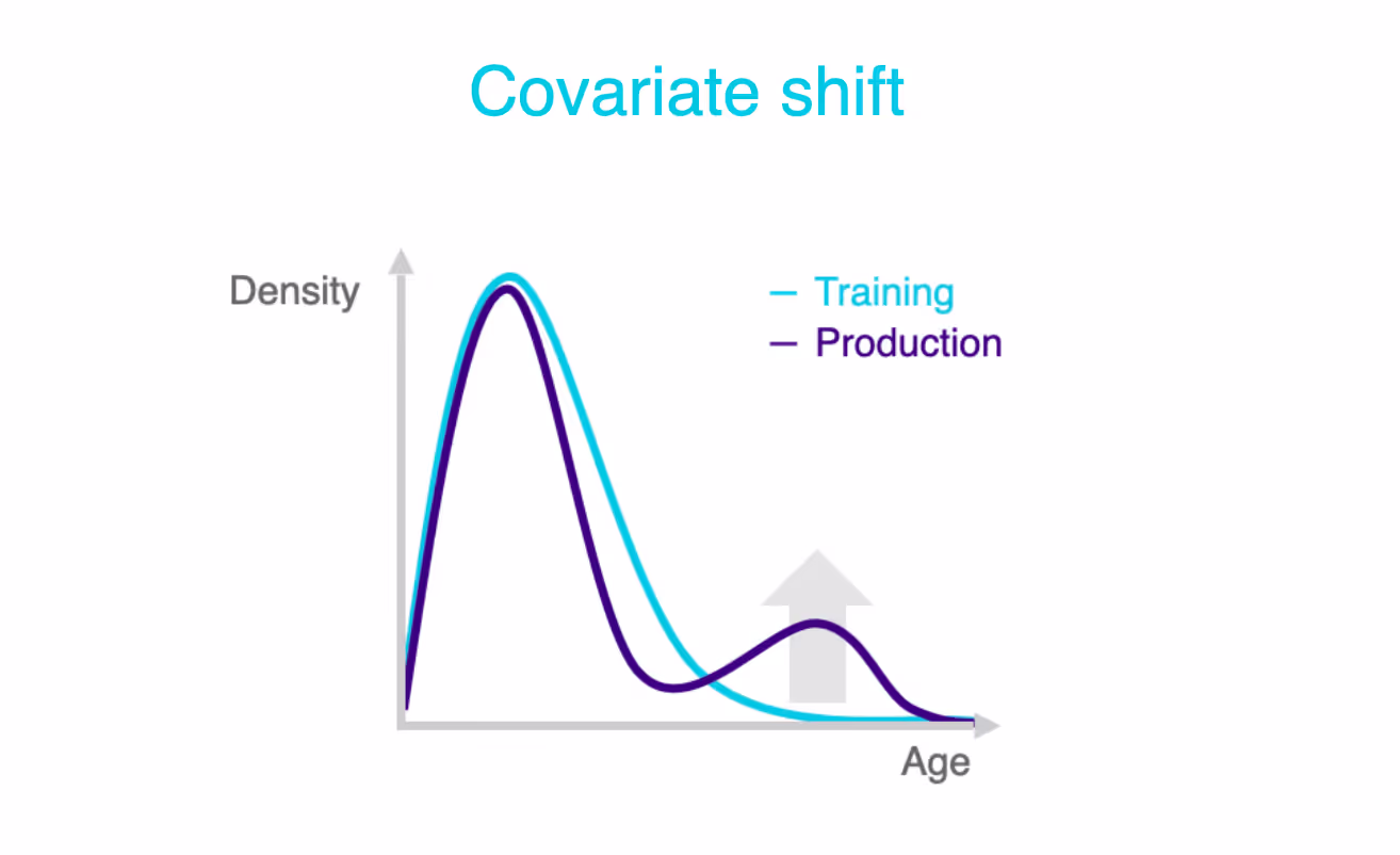
The graph above illustrates a hypothetical scenario of customer lifetime value (CLV) prediction for a social media platform. The distribution of the training data was heavily skewed toward younger customers. However, when the model was deployed in production, the distribution shifted, with a small spike in older customers.

One possible explanation for this discrepancy is that when the training data was collected, most of the platform's users were young. As the platform grew in popularity, older customers began to sign up. The characteristics of this new group of users are different from the historical ones, which means that the model is now prone to make mistakes.

The detection of data drift is relatively straightforward. We need to compare distributions from different periods to identify changes in the data. The tricky part is that not every drift leads to a decrease in performance.

Sometimes, shifts in the data may not affect the overall performance of the model. This is because not every input feature contributes equally to the output. Only shifts in important features will have a significant impact on the overall performance of the model.

To learn how to check if the data drift in your model has affected performance, read this blog next.

Concept Drift

A model can also fail to make accurate predictions if the relationship between model inputs and outputs changes - in the presence of concept drift.

The relation between CLV and Age feature for training and production data.

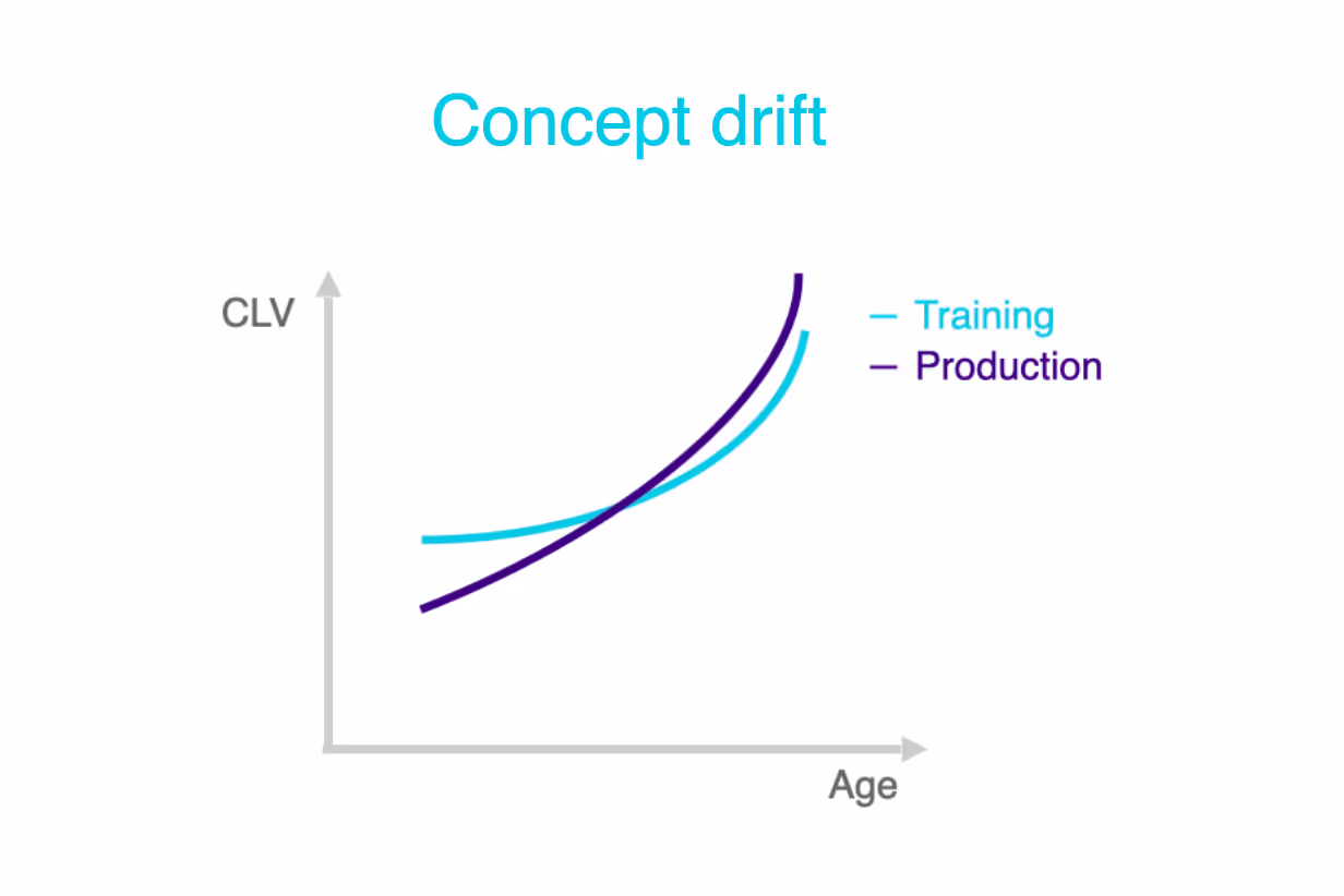
Let's get back to the example of the customer lifetime value prediction. As we can see, the CLV for younger customers decreased in production. It might be caused by the migration of younger users to the other social media platform like we saw the rapid switch from Facebook to Instagram. The relation between age and CLV extracted in the training time is not relevant in production anymore.

Unlike covariate shift, concept drift almost always affects the business impact of the model. What makes it even more challenging is that it's not easy to detect. One possible solution is to perform a correlation analysis on the labels or to train and compare two separate models on an analysis and reference period. Another approach is to carefully monitor changes in the performance of the model over time. If the performance decreases, it may indicate that concept drift is occurring.

However, monitoring the performance of a model is not always easy, especially when access to target labels is limited. We will dive into this key challenge in more detail in the next paragraph.

How the availability of Ground Truth impacts the ease of monitoring ML models

As previously mentioned, having access to the target values is a crucial aspect of monitoring machine learning models in production. Based on the availability of these values, we can distinguish three types:

1) Instant Ground Truth

Ground Truth is immediately accessible.

A typical example of instant availability is the car plan arrival estimation. After completion of the trip, we can immediately evaluate the prediction and get the real-time performance of the model.

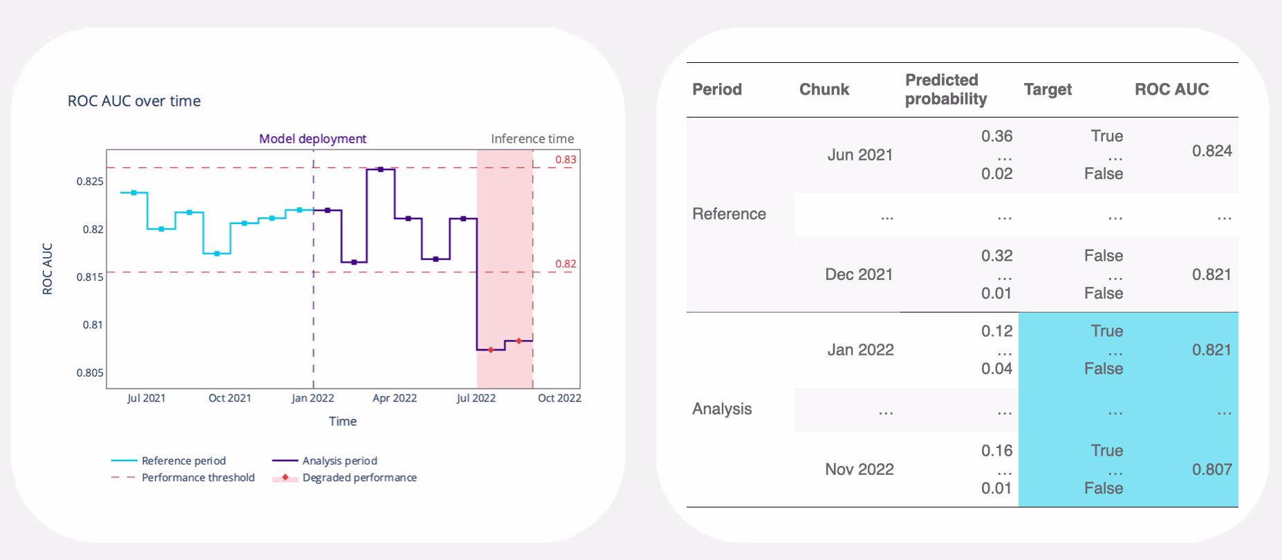
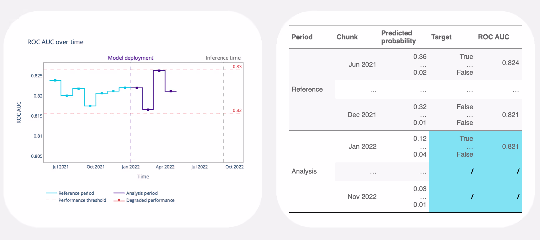
Performance Monitoring with Instant Ground Truth in NannyML and example dataset.

The graph above illustrates a common scenario in classification problems, where the reference period represents a testing dataset, and the analysis period represents a stream of data from production. On the right side, we can see an example of tabular data with the highlighted target values. With instant access to the ground truth, we can constantly monitor the performance of our model. If the performance drops below a certain threshold, as seen from June to October, this is an indication that we need to investigate the cause of the decline.

Instant access to the target values makes monitoring and evaluating the performance of our model much easier. However, the world is a complex place, and getting instant ground truth is not always so easy.

2) Delayed Ground Truth

Ground Truth is postponed in time.

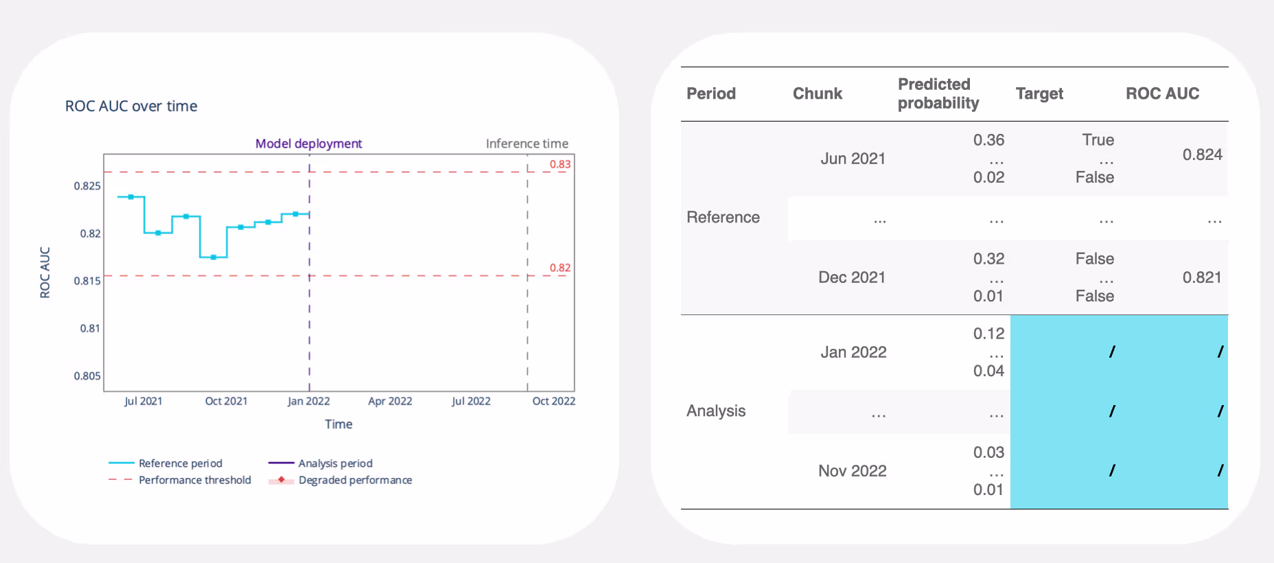
Demand forecasting for a clothing company is a great example of a scenario where ground truth is delayed. These companies use machine learning models to predict demand for the next season. However, evaluating the predictions is tricky since they have to wait three months until the season is finished to measure the accuracy of the predictions.

Performance Monitoring with Delayed Ground Truth in NannyML and example dataset.

As you can see on the right-hand side, our tabular data needs are missing target values due to delays. This lack of information is reflected in the graph, where we can see a gap in the ROC AUC performance of the model from May to November. In this scenario, it is challenging to understand how well the model performs and whether its decisions are still accurate.

3) Absent Ground Truth

No access to ground truth at all.

Ground truth may not be available in some cases, such as fully automated processes. An example is the use of machine learning models for insurance pricing. These models are deployed in production to predict the price of insurance based on demographic or vehicle information. However, since the process is automated, there is no human in the loop to evaluate the accuracy of the predictions.

Performance Monitoring in the Absence of Ground Truth in NannyML and example dataset.

As we look into the tabular data, we see that the target values are completely missing. It's shown in our performance graph, which is blank after deployment. In this scenario, it is tricky to get a clear picture of how well our model is doing and whether its predictions are reliable.

Although the lack of ground truth may sound bleak, the model's performance can still be evaluated. Even if a model doesn't have target values, it still produces output that we can compare to previous data. It is enough information to estimate its performance. While the availability of ground truth makes evaluating a model's performance easier, it's still possible to do so in its absence.

Conclusions

As a data scientist, one key responsibility is ensuring the entire model and pipeline run smoothly. However, this can often be a challenging task, as several obstacles can arise in the production, like:

code - model fails to predict due to errors/bugs

data - covariant shift or limited access to the ground truth

But don't worry; now that you know what to look out for and why they happen, you'll be able to tackle them easily.

What makes model monitoring in production hard?