Reverse Concept Drift Algorithm: Insights from NannyML Research

Do not index

Canonical URL

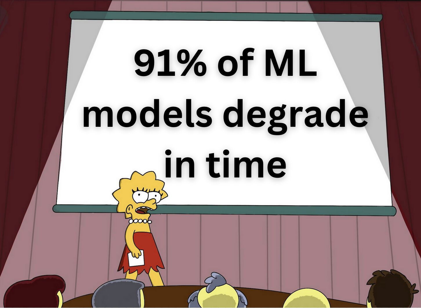
When machine learning models are deployed in the real world, their performance often diminishes—a reality faced by 91 percent of models over time. This shift has led data scientists to focus not just on building and deploying models but on actively monitoring them.

Post-deployment data science revolves around maintaining production-grade models as the data they encounter continues to evolve. It primarily deals with three issues: covariate shift, concept drift, and data quality.

This blog explores concept drift and how it impacts machine learning models. We'll discuss the algorithms and experiments we conducted to detect and measure its impact, and how we arrived at the Reverse Concept Drift Algorithm.

Concept Drift

Concept Drift develops when the conditional probability P(Y|X) changes over time while the distribution of the input features P(X) remains constant.

Think of a beauty product recommendation system that initially suggests products based on user preferences and past purchases. This model performs well when it’s first deployed, accurately recommending items that users appreciate. However, new trends emerge over time, such as a growing demand for eco-friendly and natural products. These changes in user preferences mean that the model’s initial understanding of what users like is no longer valid.

This shift in preferences is quantified as concept drift. It occurs when the relationship between input features (user preferences) and the target outcomes (product recommendations) changes, even though the distribution of features (user data) remains the same.

In simple terms, the model’s learned patterns become outdated.

Our Research

1. Naive Residuals

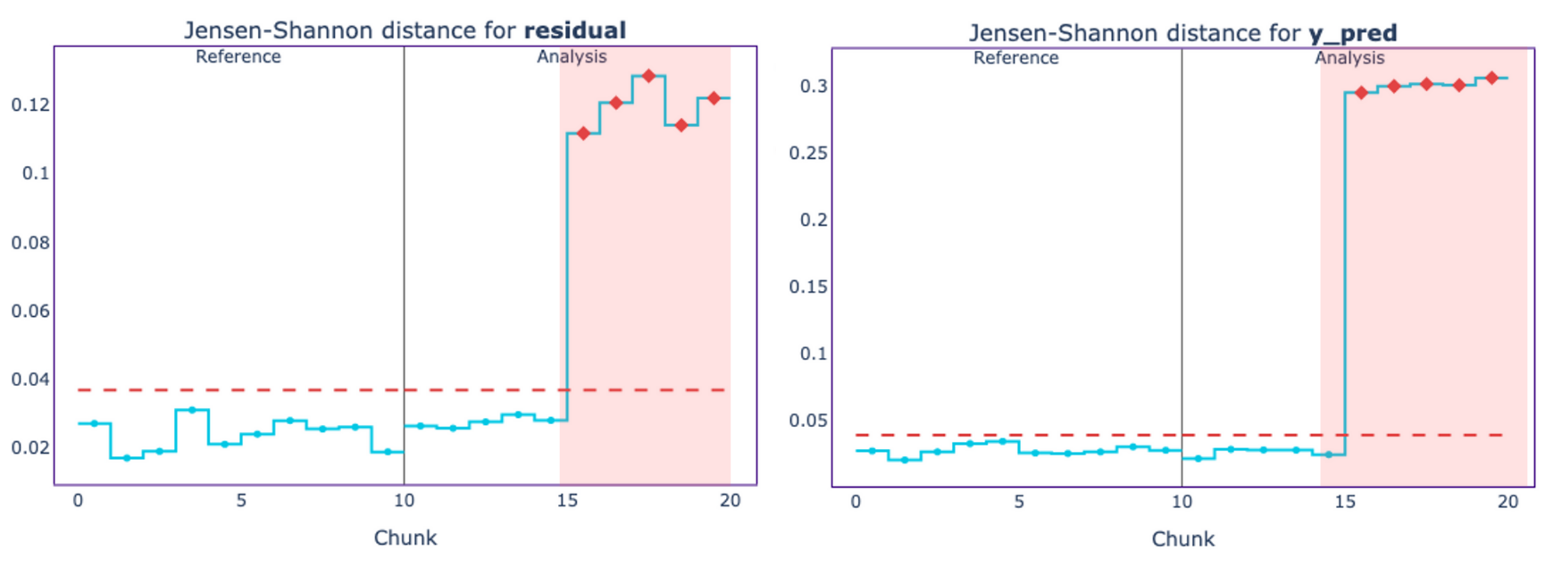
When thinking about concept drift, the first approach that often comes to mind is analyzing residuals.

Residuals are computed by subtracting the predicted values from the actual values for the reference and analysis datasets.

What are reference and analysis datasets?

NannyML requires your data to be formatted into reference and analysis sets. The reference dataset is representative of optimal or benchmarked version of model performance. For newly deployed models, it is the testing dataset. The reference data is compared against the analysis or monitored dataset. This dataset is representative of the current state of production data.

The goal here is to calculate residuals and use them as a univariate signal to monitor potential concept drift. This helps understand how well the model's predictions align with the actual values. Large residuals can indicate potential issues like concept drift.

reference_df['residual'] = reference_df.y_true - reference_df.y_pred
monitored_df['residual'] = monitored_df.y_true - monitored_df.y_pred

This method, while intuitive, is only a starting point. Residual analysis can give a quick snapshot of potential shifts in the concept. Still, it doesn't capture the full complexity of concept drift, especially when factors like covariate shift and interaction effects are in play.

Univariate Drift Monitoring on Residuals. The cause of these alerts could be covariate or concept drift.

💡

NannyML OSS python package brings post-deployment data science into your workflow with just one pip install.

If the user base changes (covariate shift), such as more younger users joining, the recommendation system might start favoring products popular with this group. If user preferences shift (concept drift), such as a growing preference for eco-friendly products, the system would adapt to recommend more items.

If the user base and preferences change simultaneously, their effects might cancel each other out. Younger users might prefer the same products as before, even if the overall preference for eco-friendly items increases. In this case, the system might not show a noticeable shift in recommendations.

If the preferences of a particular user base are changing while the user base itself is also evolving, the combined effect might mask the true nature of the changes.

Do you see how separating these shifts is important?

2. Resampling Residuals

To further understand and quantify concept drift, we explored resampling residuals as an analytical approach. This method aims to isolate the effect of concept drift by minimizing the influence of covariate shifts in our data.

Resampling monitored data so that its distribution is similar to that of reference data is a computationally expensive process.

Given the complexity of matching multidimensional distributions, we simplified this process by aligning the distributions based on y_pred_proba , at the cost of losing accuracy. This approach seeks to find the closest matches between the reference and monitored data by minimizing differences in predicted probabilities.

After resampling, the residuals from the monitored data (with the covariate shift effect removed) were compared to those from the reference data.

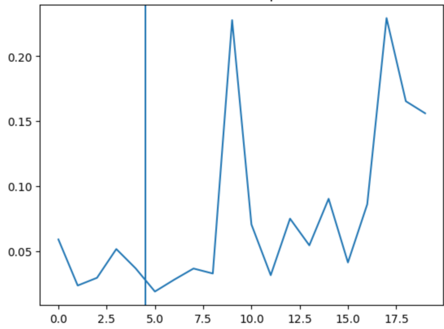
To quantify the differences, we needed a single value to summarize this drift. Instead of relying on aggregate statistics like the mean absolute residual, which may overlook distribution changes, we start with the Kolmogorov–Smirnov test.

The KS distance can reveal distributional differences but isn't easily interpretative, making it difficult to draw clear conclusions about the nature or impact of concept drift. Distance measures like this are, at best, a monotonic function of concept shift—they increase with the magnitude of concept shift, but the exact relationship between them is unknown and varies depending on the actual distribution.

This realization led us to seek alternative methods that allow for more direct measurement of integrals.

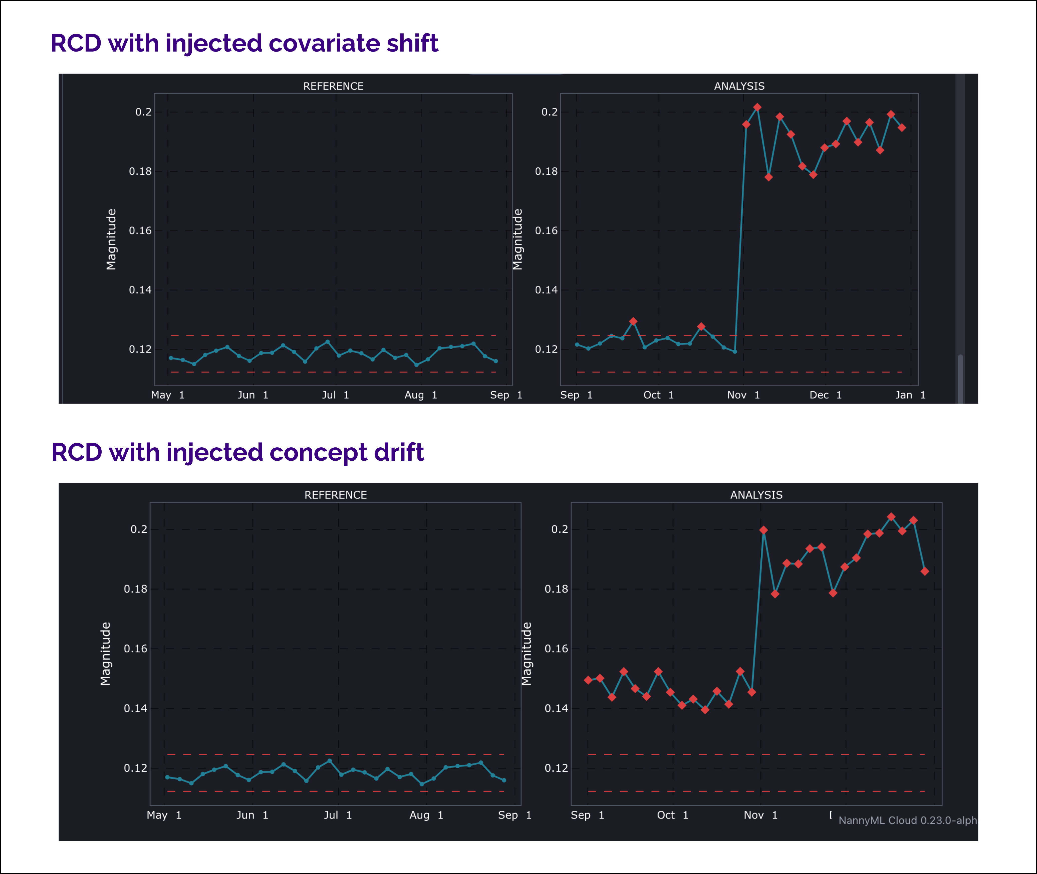
Reverse Concept Drift

One meaningful way is to use reference inputs to control for covariate shift. By focusing on reference inputs—those that are consistent and representative of the underlying data distribution—we can more accurately isolate the effect of concept drift.

This algorithm involves comparing the model's performance on the reference data to its performance on the current data, where only the concept has drifted while the covariate distribution remains controlled.

If drift is present, then a concept is present in monitored data but not in reference data. This means a new model can be trained to learn the updated concept and compare it to the old model. Using the concept from monitored data with the reference dataset, we can see how predictions would look if the reference data had a new concept.

Implementation

Train on New Data: Start by training an internal model on a recent dataset to capture any new concepts that may have emerged.

Predict on Reference Data: Apply this internal model to the reference dataset to generate predictions.

Estimate Performance: Evaluate the model's performance on the reference dataset, treating the internal model's predictions on the monitored data as the ground truth.

Compare Results: Assess whether there is a significant difference between the internal model's performance and that of the actual model. A notable discrepancy indicates that concept drift has occurred.

💡

We refer to this as Reverse Concept Drift (RCD) detection because it involves using analysis for model fitting and reference data for prediction.

Magnitude Estimation (ME) measures the extent of concept drift by quantifying the difference between the model's concept on monitored data and the reference data.

As ME increases, performance is anticipated to drop. However, there isn't a direct one-to-one correlation, so ME alone cannot be relied upon entirely. To connect concept drift with business impact, we need to measure how drift affects model performance.

We can achieve this with the Performance Impact Estimation metric. It is the difference between the actual model's performance on the reference data and the estimated performance based on the internal model. The calculation assumes that the new comparison model’s predictions are the ground truth for the reference set and the predicted scores are well-calibrated probabilities.

PIE and ME metrics on an example dataset. An increase in ME does not have a direct correlation with performance. Considering both metrics is important.

The chunk size for comparison must be sufficiently large, around 1000. A large amount of data ensures that the density ratio estimation model can be accurately trained and properly multi-calibrated.

Drawbacks

Reverse Concept Drift usually effectively manages covariate shifts. However, it can struggle in extreme cases. Consider our recommendation system again: If user demographics change drastically and new user groups arrive that were not present in the reference data, RCD may face issues. If these new user groups are missing, the concept learned from the remaining data might not reflect the true concept.

Relationship between Concepts and Covariate Distribution

RCD relies on the reference data covering the same input space as the monitored data. Practically, if we don't have data from an analysis region in the reference data, we can't account for that shift with a weighted calculation from reference data.

This limitation means the model might learn an incomplete or incorrect concept, leading to inaccuracies.

The Reverse Concept Drift Algorithm treats covariate shift as concept drift because it mistakes it as a new concept.

Conclusion

Data scientists know that the real challenge begins after model deployment. Monitoring models in production is non-negotiable to maintain their relevance and performance.

Our exploration of concept drift, from residual analysis to the Reverse Concept Drift algorithm, is a small part of our journey to solving post-deployment issues.

NannyML Cloud helps you monitor your models without ground truth and stay ahead of drift. Schedule a demo with NannyML founders today to discuss tailored solutions for your use case.

What’s next?

Now that you understand concept drift and how to detect it, you might wonder how to address it. The first prompt is to retrain regularly; however, I recommend you read this blog to evaluate that notion.

Retraining is Not All You Need

Your machine learning (ML) model’s performance will likely decrease over time. In this blog, we explore which steps you can take to remedy your model and get it back on track.

https://www.nannyml.com/blog/retraining-is-not-all-you-need

If you want to learn about other algorithms we've developed, look at these.

Estimating Model Performance Without Labels

Blogs about all things data science and machine learning, post deployment. Most popular topics: data drift, model monitoring.

https://www.nannyml.com/blog/machine-learning-performance-estimation

Multivariate drift detection using Domain Classifier with a Python tutorial

A comprehensive explanation and practical guide to using the Domain Classifier method for detecting multivariate drift.

https://www.nannyml.com/blog/data-drift-domain-classifier

Frequently Asked Questions

How do we test for concept drift?

Reverse Concept Drift Algorithm detects concept drift and quantifies its performance on model monitoring performance.

What is the equation for concept drift?

Concept drift is expressed as a change in the conditional probability distribution P(y∣X). The equation quantifies the difference between the current and reference distributions, reflecting shifts in the relationship between model inputs and targets.