How to Set Up a Machine Learning Monitoring System

Do not index

Canonical URL

In the world of machine learning, almost every data science project starts with an exploration phase in the Jupyter notebook. After extensive training and testing, the model is ready to be elevated to production. Then it's integrated into the deployment pipeline and hosted as an API. Although this may seem like the end of the journey, an essential component is still missing: a monitoring system.

In this blog, we dive into the process of setting up a monitoring system using NannyML with the support of three tools - Grafana, PostgreSQL, and Docker. With their help, you can make sure your machine learning model keeps delivering business value and have the impact you'd signed off on.

So buckle up, and let's get into it!

Context

Demo use-case

A recent study published in Nature has revealed that 91% of machine learning models suffer from performance degradation in production. So, unfortunately, your machine learning model will likely experience this issue. But there is a light at the end of the tunnel: the constant monitoring of its performance.

Performance monitoring can be challenging, mainly when the ground truth is not immediately available. However, NannyML can estimate the model's performance based on input data and its predictions, even when the target value is delayed. In the following paragraphs, we'll dive into a monitoring system with estimated performance for car price prediction.

We'll use a synthetic dataset created explicitly for this purpose to demonstrate this system. The model's task is to predict a used car's price based on seven different features.

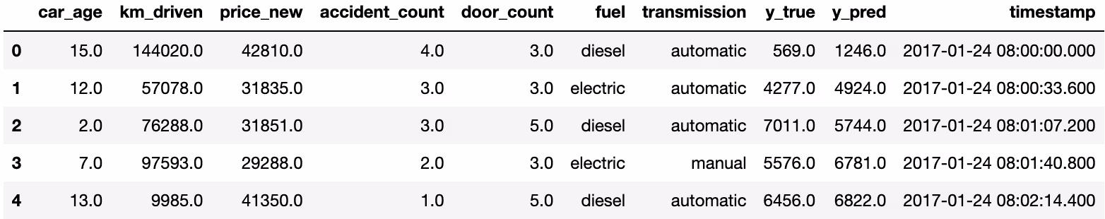
First 5 rows of car price prediction dataset.

This is a snippet of our data where y_true is an actual target value, and y_pred is a model's prediction. The dataset is split into two sets:

reference - testing data and predictions

analysis - production data and predictions

You can find more detailed information about the dataset in the docs.

To mimic the production environment, we will simulate the daily run of NannyML. Don't worry; the process will be faster than it sounds. We will speed it up so a day's worth of data will appear every minute on our Grafana dashboard.

Also, as a bonus, we will set alerts up in Grafana with notifications in Slack.

Monitoring System in Production Environment

The following image is an overview of the machine learning model lifecycle stages, including development and deployment. Initially, the model gets trained and tested before being implemented as a predictive service in a production environment.

In this context, we will focus specifically on the Monitoring System aspect and its parts:

NannyML - the core of the operation, it takes the testing(reference) and production(analysis) data and returns the performance estimation and drift detection calculations.

PostgreSQL - a database that stores the outputs from NannyML.

Grafana - the dashboard visible in the browser, where we can monitor our performance and drift detection.

Docker - the underlying software that bonds altogether, allowing us to run our application with just one command. If you want to understand the basics of Docker, check out this article.

Requirements

The only thing we need to download and install is Docker. Here's a link with the instructions on how to do it.

Now that we've gone through the entire system, its components, and requirements, it's time to roll up our sleeves and dive into the repo itself! Let's get started!

Code walkthrough

💡

Note: The demonstrated snippets of the code are tailored for Mac and may differ on Windows, although the Docker commands and outputs should be the same.

1. Clone the repo

The first step is to go to NannyML's GitHub link and to git clone the examples repo.

$ git clone https://github.com/NannyML/examples.git

As previously stated, our focus is on the regression example in which data is received every minute. That's why the directory for this example is named regression_incremental. Additionally, the repository includes other examples, such as binary and multiclass classification and regression, but the data for these cases remains static.

$ cd regression_incremental

2. Configuration Files

Before running Docker, it's good to see what we are setting up. In our directory, there are two important configuration files:

1. NannyML - nann.yml

First let’s take a closer look at it in command line:

$ cat nannyml/config/nann.yml

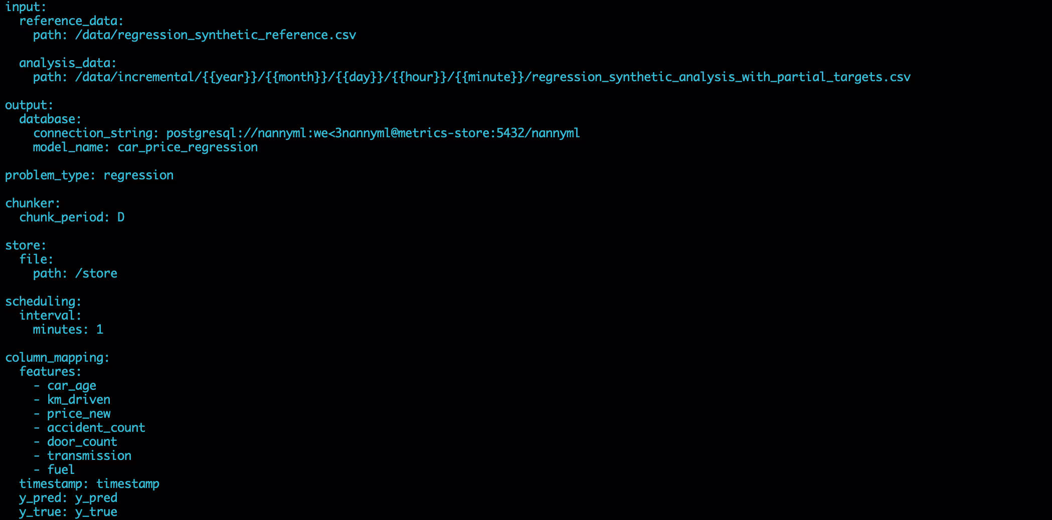
As we can see here, there are multiple essential sections to specify for your project, like:

input - inputs for NannyML read from /data directory

reference data - path for the reference set
analysis data - templated path for the analysis set, to ensure that you read file from the specific year, month, day, and minute

output - defines where we write the results

connection_string - configures where and how to connect to PostgreSQL
model_name - it’s useful when we are monitoring multiple models, and we want to watch them at the same dashboard

problem_type - type of use case we are working on

chunker

chunk period - refers to the division of data into parts or segments. In our context, D represents a daily split, meaning each chunk period is equal to one day.

store

file and path defines where we store the performance estimators

scheduling - defines how often we are running the NannyML, for the demo purposes we set it to one minute

column_mapping - specific information about the input features

2. Docker - docker-compose.yml

$ cat docker-compose.yml

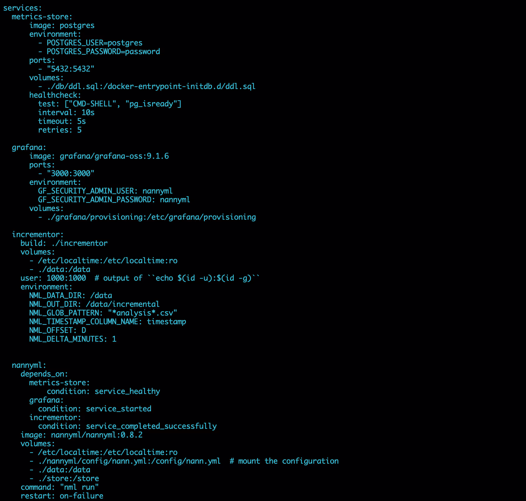
Terminal screenshoot of docker-compose.yml file.

This file is all setup and good to go. We are taking a look at it to understand better the containers that Docker is setting up:

metric-store - a PostgreSQL container providing the database for storing the NannyML’s outputs

grafana - a Grafana container that connects to the metric-store, and display it in the dashboard

incrementor - a custom built container running a Python script that will take the analysis data, group it per day and write each group in a directory following the template used above.

nannyml - The NannyML container processing the calculations

3. Run the Docker

docker-compose up is a command used in Docker to create and start containers for each service, defined in a docker-compose.yml file. It makes it easy to run, test, and debug an application without worrying about the underlying infrastructure and dependencies.

Finally, let's bring all our containers alive:

$ docker compose up

Execution of docker compose up command in terminal.

When you execute this command, you'll see a lot of output, but once you spot the NannyML logo, it indicates that the first run started. After it's finished, we should see our results on the dashboard.

Understanding how nannyML can integrate with your monitoring solution? we can help you get started. Talk to one of the founders who understand your use case

4. Grafana

Connection

Our Docker is running and we can see how the model is performing in Grafana. To see the dashboard, open up the browser and go to http://localhost:3000. Now, log in using the username nannyml and password nannyml .

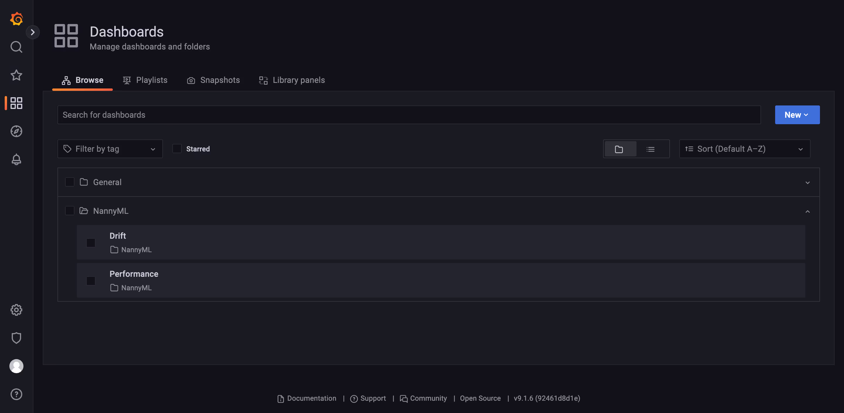
Dashboards

In the navigation menu on the left, there’s a Dashboard icon. To see the available dashboards, click on the Browse button.

As I mentioned before using the Grafana, we can monitor two values:

Performance Dashboard

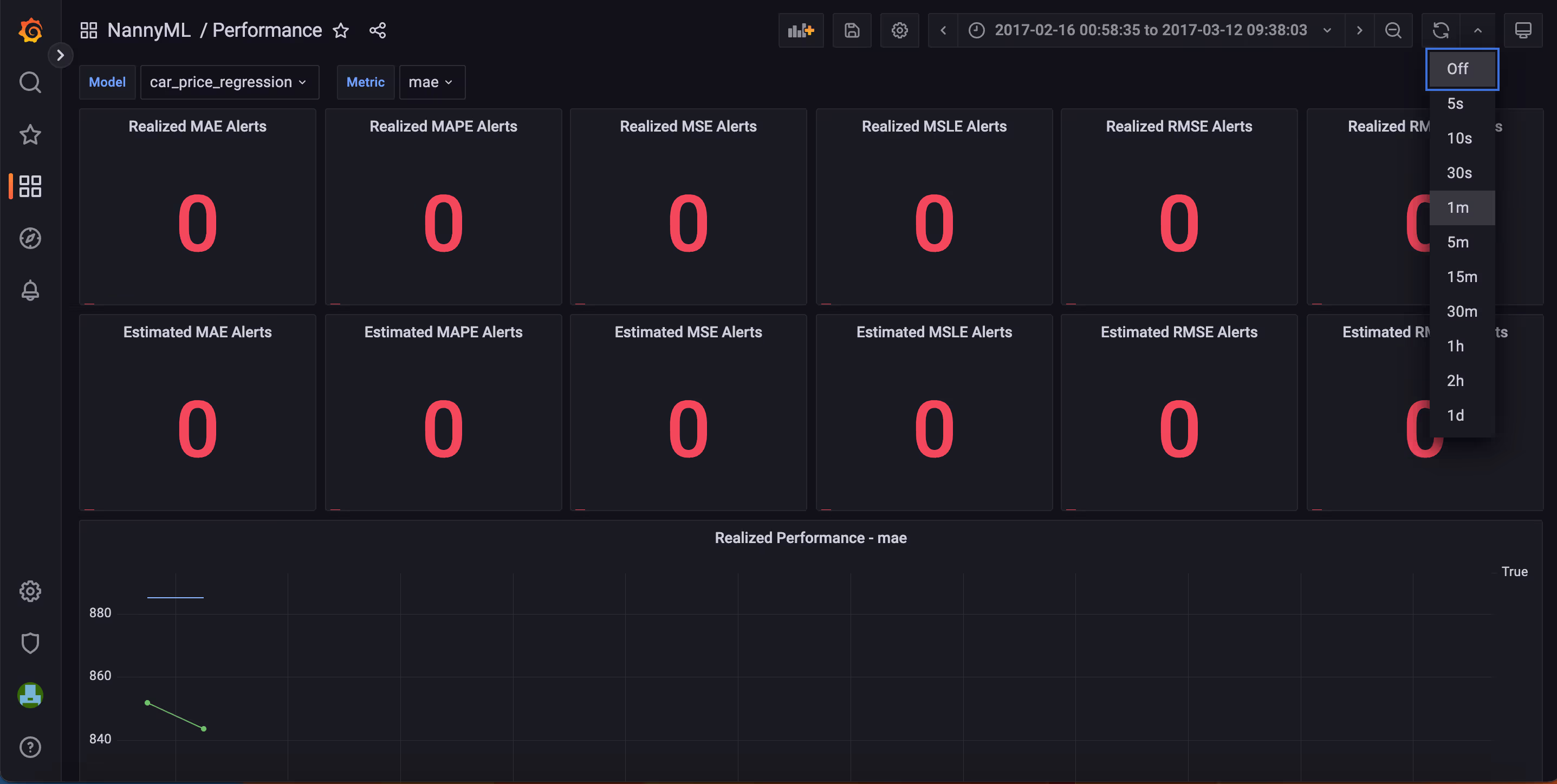
Before we dive into the analysis, it's important to change the refresh value in the top right corner to 1m. This will provide us with a real-time view of the performance.

We can see numerous alerts divided into two categories, estimated and realized. Estimated are the results of our DLE performance estimator, while realized represents the actual performance computed using the ground truth.

Additionally, Grafana offers an interactive dashboard, allowing us to arrange and customize the graphs for optimal viewing. In this instance, I only saved the alerts for the MAE metric and changed the size of the plots to make everything fit on the screen.

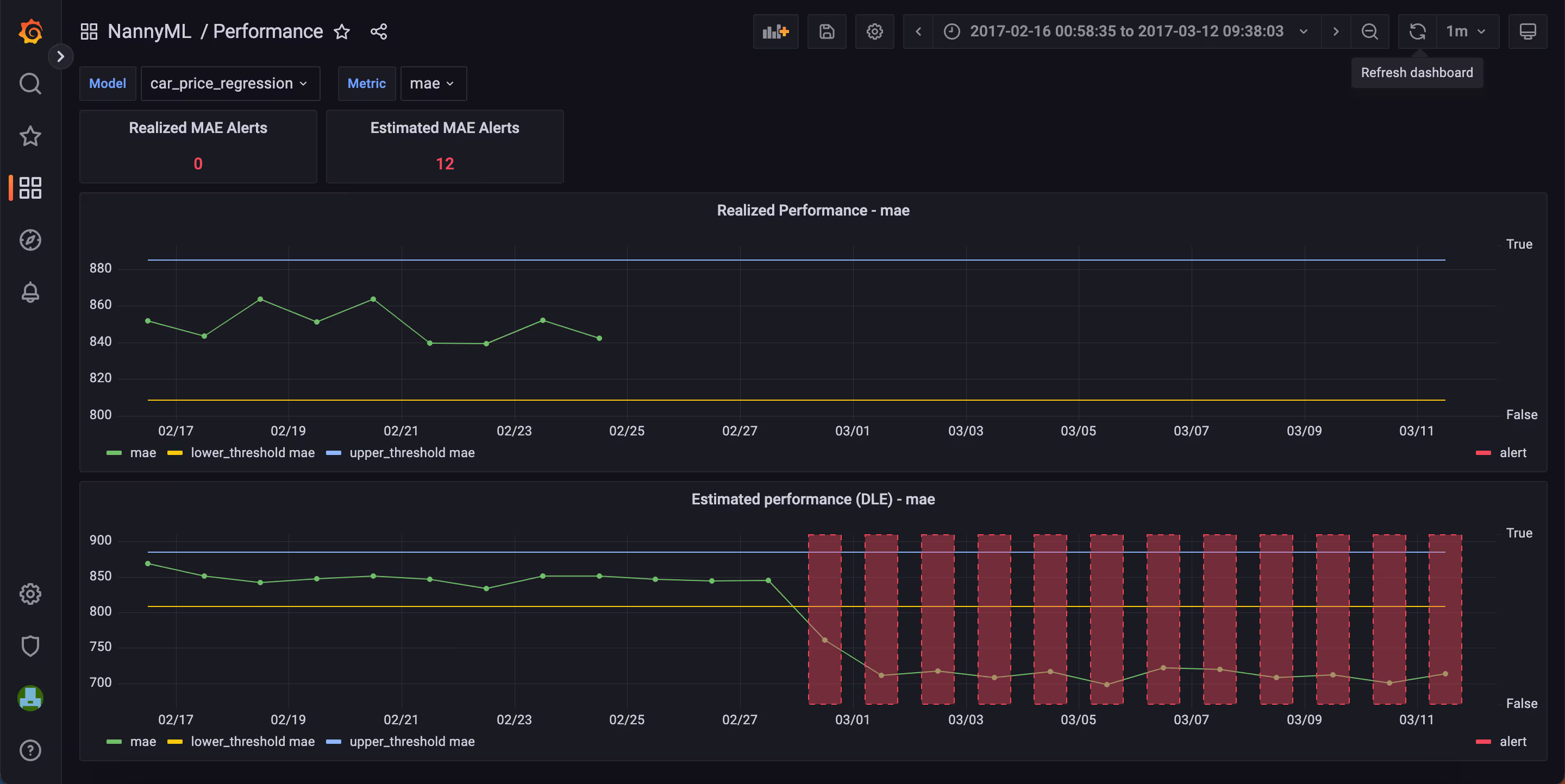
Manually customized performance dashboard.

The estimated performance has experienced a significant drop since March, leading to 12 alerts in estimated MAE. We can also observe graphs for other metrics changing the value in the Metric dropdown menu at the top.p.

Additionally, the actual performance is recorded until February 24th, while the estimated performance is still ongoing. This is due to the delayed target values, as the actual price of a car is challenging to acquire in real-life situations. Data on car prices can be collected through various methods, like tracking sales prices at dealerships, online marketplaces, or conducting surveys with experts. However, all of these methods take time, resulting in a delayed availability of the ground truth.

Anyway, we can see a persistent decline in the estimated performance. It indicates the need for additional analysis to detect data drift and find potential explanations.

Drift Dashboard

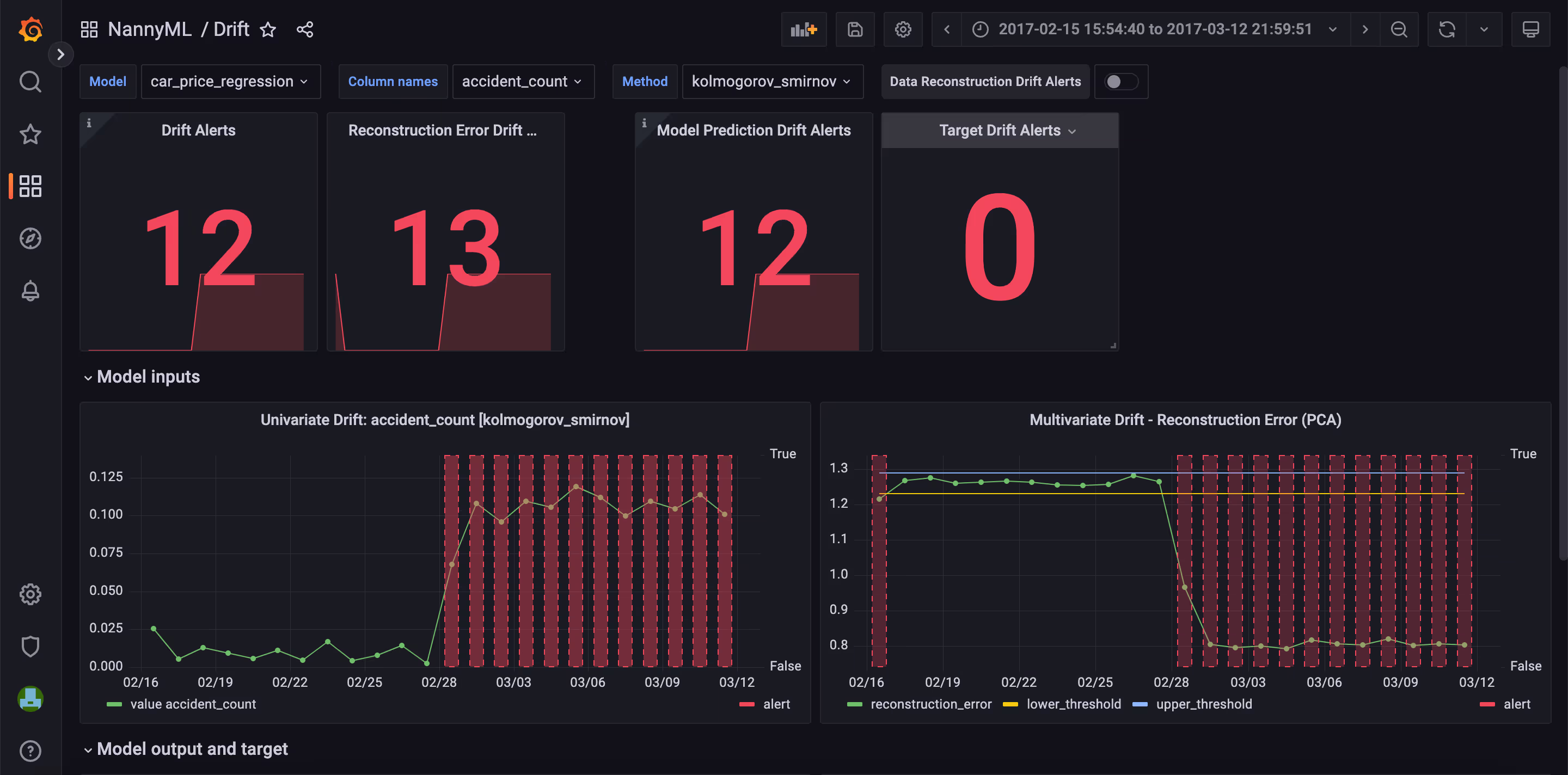
As we can observe, we ended up with numerous alerts. The results displayed above are calculated for the selected model, column name, and method. We can manipulate these values based on the results we wish to see. The multivariate drift error provides a more general view of potential data drift and clearly shows significant changes in the inputs. This drift also overlaps with the decline in the estimated performance, suggesting a possible cause.

To gain deeper insight into which feature is responsible for this, we can plot all of them on one graph.

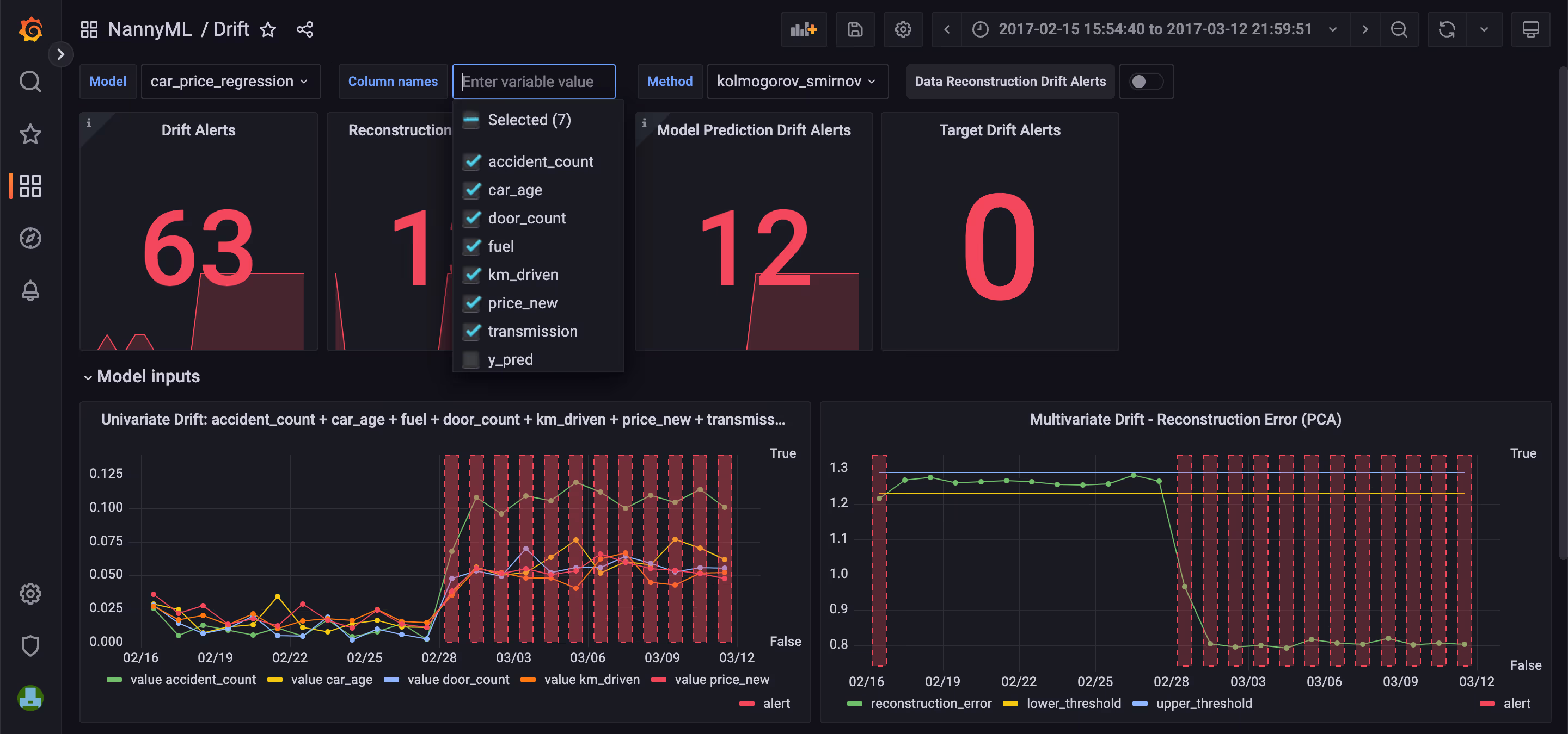
Adding more features to the drift dashboard.

In the Kologorov-Smirnov graph, the feature that has undergone the most significant drift is the accident_count. Further analysis and investigation go beyond the scope of this blog post and requires a data scientist to step in.

If you have finished working with Grafana, you could stop the container using the CTRL+C, and to entirely remove the containers, run this command:

$ docker compose down

5. (Bonus) Slack Notifications Setup

Now, we can get to our bonus part where we are setting up the Grafana Alerts along with the Slack.

Create a webhook URL for your Slack channel

Right-click on your channel and go to View channel details then to the integrations.

Now you can click on the Add an App button.

Search for incoming-webhook.

Click on view and then configuration .

The new window should pop in the browser and click on Add to Slack .

Choose a channel and click on Add Incoming WebHooks integration.

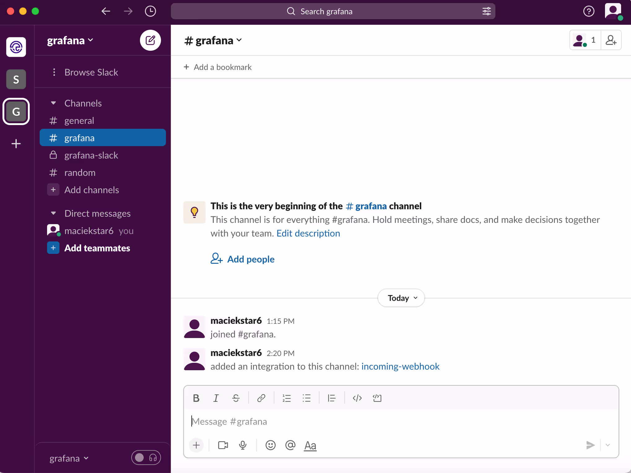
Don’t close the window in the browser, go to Slack and see if you got this message:

Screenshot from the setup channel in Slack.

Copy the Webhook URL from the browser.

Set up a contact point between Grafana and Slack

Run the docker compose up and go to Grafana : http://localhost:3000/alerting/notifications

Click on New Contact Point.

Add :

Name: Slack

Contact point type: Slack

Webhook URL: Paste your Webhook URL

Test it by clicking on the Test button next to the Contact point type, with predefine message, which should look like this:

Screenshot of testing message sent from Grafana.

Set Slack as a default Notification Policy

Go to Grafana again, and click on Notification policies next to the Contact Points.
You should see the Root policy - default for all alerts. Now go to the Edit, and change the Default contact point to Slack and Save.

Create an Alert Rule

To keep things straightforward, we will limit ourselves to setting up the Alert Rule only for the estimated performance. In other words, when the value of the alert (calculated by NannyML) reaches 1, indicating that the estimated performance is beyond the threshold, we will receive a notification on Slack.

Go to the dashboard, and edit the Estimated Performance Graph.

Then click on Alert → Create alert rule from this panel .

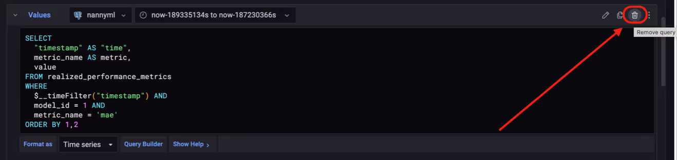
First, remove the Values and Threshold queries since we will only use the Alert one.

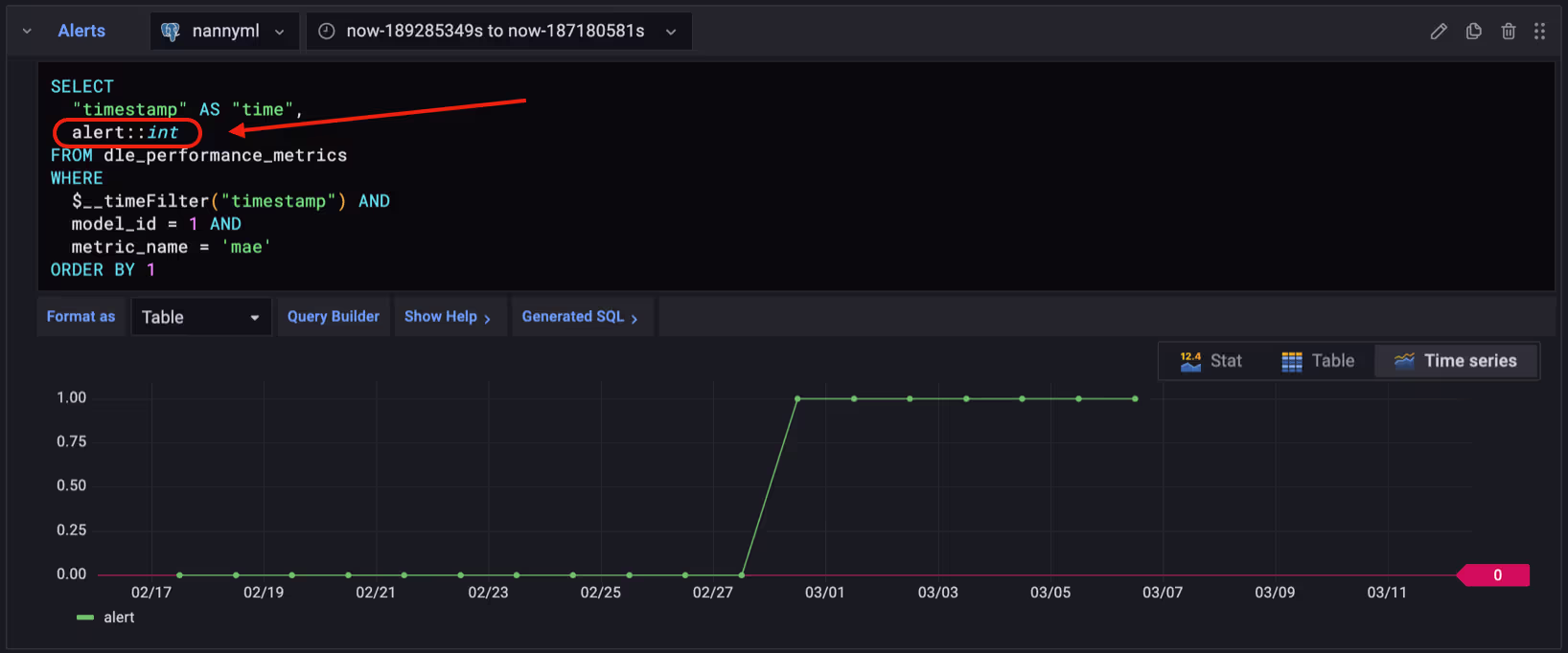
Convert the alert value to int by adding the ::int

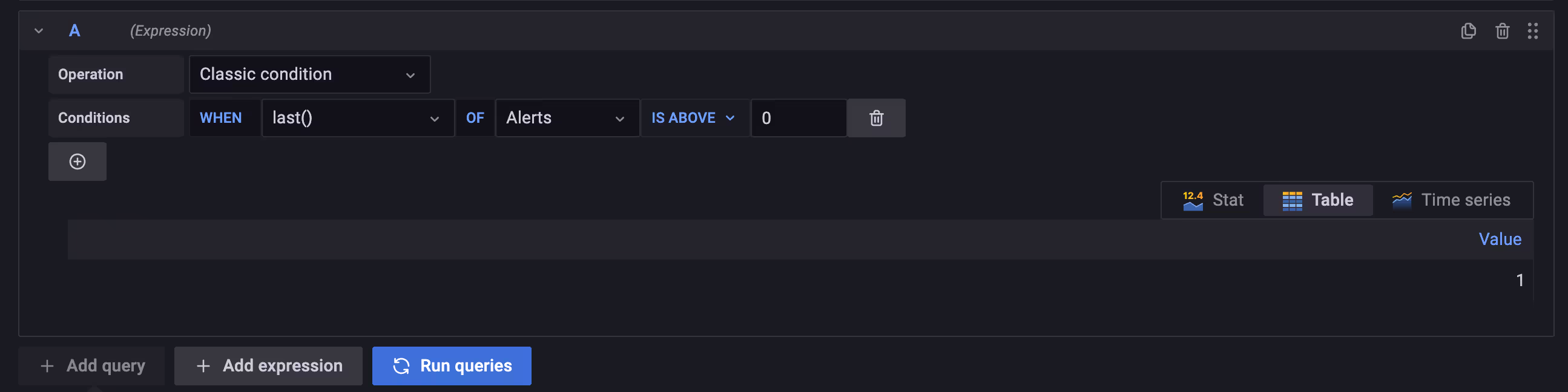
Now we can add the condition if the last value of alert is above 0(estimated performance is beyond threshold), we get the notification. Also, Run queries to make sure everything is working fine.

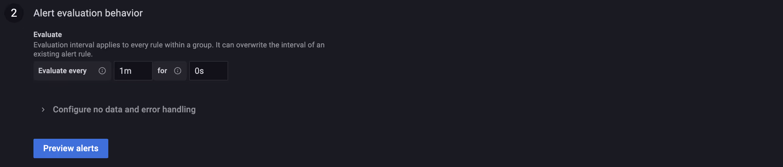
Alert evaluation behaviour, we set it to every minute, since our data comes in that schedule. The for argument is set to 0s, since we want our alert start firing straight away.

Setting up the alert evaluation intervals.

The rest will work well with default setup, just you need to put arbitrary name in the group section for the demo-purposes. Now, click Save and Exit .

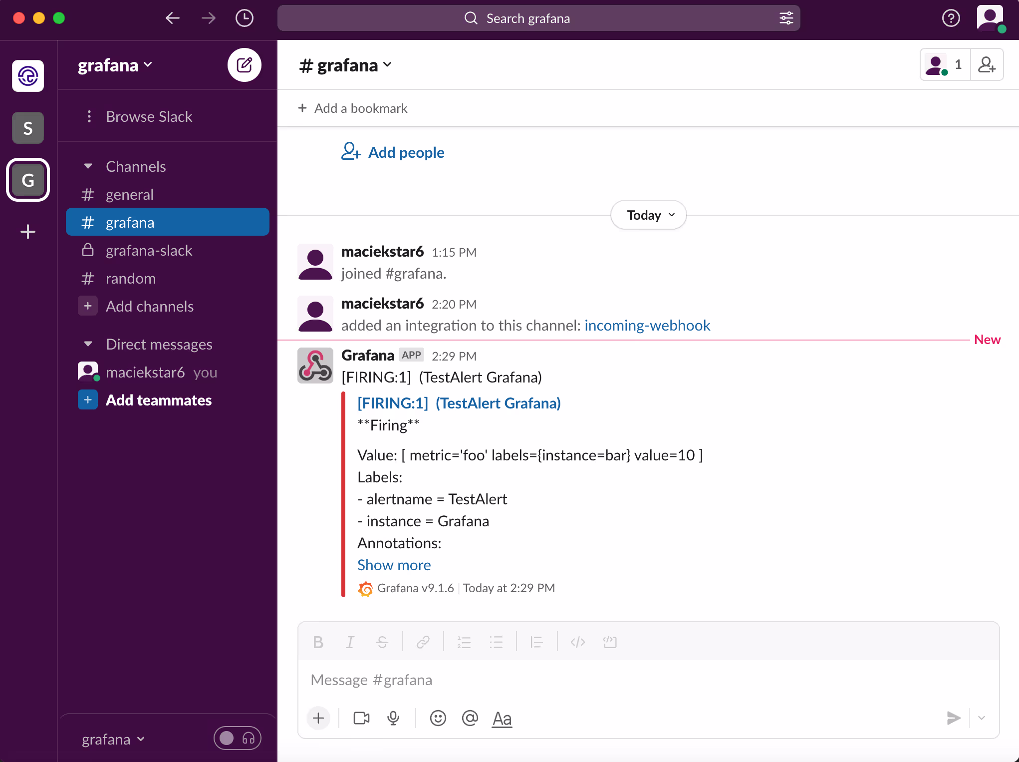
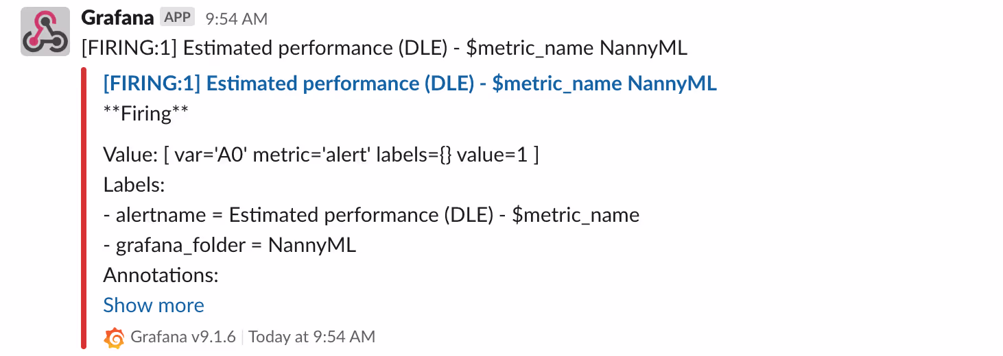
Now you should see this message on your Slack channel:

Screenshot of alert information in Slack.

Not feeling like deploying nannyML on your own? we can help you get started. Talk to one of the founders who understand your use case

Final words

Congratulations on making it to the end! By now, you have gained a good understanding of the process of deploying NannyML in production. You have learned about the significance of a monitoring system and the different components required for its implementation, including the configuration files for Docker setup. You have also gained knowledge on how to navigate and utilize Grafana, as well as how to integrate it with Slack to receive alert notifications. Now you're fully equipped to experiment with this setup on your own and incorporate it into your system!

How to Deploy NannyML in Production: A Step-by-Step Tutorial