Multivariate drift detection using a real world dataset

Do not index

Canonical URL

Imagine investing significant resources in designing and deploying a machine learning model, only to discover that its performance has deteriorated. Covariate shift, among other types of data drifts, is a primary cause of model degradation. It can majorly impact business outcomes, resulting in financial losses, lower customer satisfaction, and reputational damage. This blog introduces covariate shift and various approaches to detecting it. It then deep-dives into the various multivariate drift detection algorithms with NannyML on a real-world dataset.

But What is Covariate Shift?

Geometrically, the distribution of the input features in a multidimensional space would look like a data cloud. A covariate shift occurs when this shape changes due to variations in the input features.

In most real-world machine learning environments, a covariate shift indicates that the characteristics of the data during the training period do not perfectly match the characteristics of the data the model encounters during production. This is a common occurrence. If this mismatch is not addressed, the model struggles to generalize to the new, unseen data and thus begins to fail silently.

Multivariate and Univariate Detection Methods

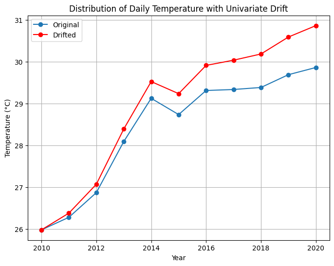
A change in the distribution of a single variable or feature over time is referred to as univariate drift, for example, in a dataset that records a city's daily temperature over several years. Univariate drift occurs when the temperature attribute rises or falls throughout the production phase. The model, however, remains unexposed to any such change since its training data is older. This can be defined as the movement of data points along a single axis, as seen in the figure below.

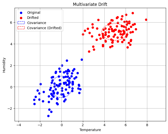
Figure 1: Graph explaining univariate changes using a synthetic dataset

If the dataset contained more variables, like humidity or pollutant levels, the chances of a multivariate drift would be higher. Multivariate drift involves a change in the joint distribution of multiple variables over time. Geometrically, this would be represented by the points changing shape, orientation, or position in the multidimensional space, similar to the figure below.

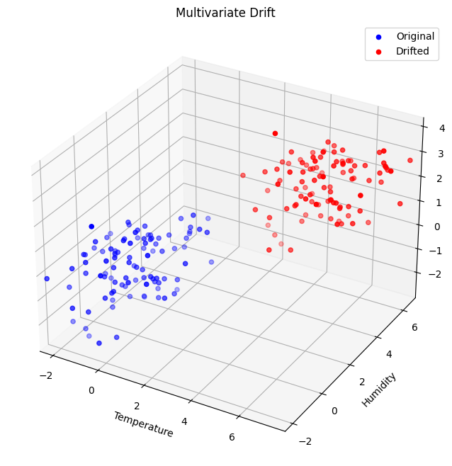
Figure 2: Graph depicting multivariate changes with a synthetic dataset.

Figure 3: A 3-D Graph depicting multivariate changes with a synthetic dataset.

Now that we understand all the key causes, we can proceed with multivariate drift detection algorithms.

Multivariate Drift Detection Methods

Multivariate drift detection methods analyze changes in the relationships between several variables or features in a dataset over time. It essentially looks for changes in the overall structure of the data that can influence the performance of machine learning models.

Figure 4: Types of Multivariate Drift Detection Algorithms in NannyML

NannyML has developed two key algorithms: Data Reconstruction using PCA, which evaluates structural changes in data distribution, and Domain Classifier, which focuses on discriminative performance.

Data Reconstruction with PCA

Principal Component Analysis (PCA) is a technique that determines the best features while lowering the dimensionality of data. It achieves this by finding the axes (principal components) that best represent the spread of the data points in the original feature space. These axes are orthogonal to each other and capture the directions of maximum variance in the data. PCA creates a new feature space that retains the most significant information by projecting the data onto these axes.

This notion of PCA is used to detect data drift. As the underlying structure evolves, the dataset will drift, and the older main components may no longer be effective at catching new trends. The algorithm detects this by comparing the original dataset to a compressed version based on the principal axes. If the compressed version differs significantly from the original, it indicates that the relationships between the variables have changed, implying drift.

Imagine you have a blueprint of your original data, and you try to recreate it using only the principal components. The difference between this blueprint and the actual dataset is called the reconstruction error. Technically, reconstruction error measures the discrepancy between the original data and its reconstructed version. This reconstruction is achieved by projecting it back into the original feature space from the lower-dimensional space defined by the principal components.

The higher the drift, the greater the variance between the original and decompressed data and, consequently, the larger the error term.

The reconstruction with PCA algorithm has the following steps:

Data preparation for analysis includes addressing missing values, encoding categorical information, and scaling the data.

Dimensionality reduction with PCA captures the major variance in the data.

During the decompression and error calculation step, the compressed data is stretched back to its original dimensions, and the reconstruction error is calculated. This error measures how closely the reconstructed data matches the original, providing insights into any changes or discrepancies in the dataset.

An alternative to the data reconstruction method is the domain classifier algorithm, which provides a finer-grained analysis by focusing on the differences between datasets during the training and production phases.

Domain Classifier

The domain classifier detects drift by training a classifier to distinguish between reference and analysis datasets. The classifier's performance determines how different the two datasets are. I will discuss the reference and analysis datasets in more detail later in the blog.

The domain classifier learns to draw a boundary in the feature space that best separates the points in the reference dataset from those belonging to the analysis dataset. This boundary is created by comparing the values of the features in both datasets and finding the optimal way to distinguish between them. The classifier is then evaluated using AUROC. If the metric is near 1, the classifier can easily distinguish between the two datasets, implying a change in the analysis set. An AUROC value of 0.5 is more desirable as it implies that the classifier is not able to discriminate between the two datasets, suggesting no significant covariate shift has occurred.

Hands-On Tutorial with NannyML on Air Quality Dataset

Importing Dataset and Setting Up Environment

NannyML is a complete Python library designed specifically for machine learning monitoring. It offers a wide range of tools and algorithms to help data scientists detect and manage drift in their machine-learning models.

💡

If you're interested in evaluating NannyML as your ML monitoring solution, I highly recommend checking out the full guide here:

Guide: How to evaluate if NannyML is the right monitoring tool for you

Blogs about all things data science and machine learning, post deployment. Most popular topics: data drift, model monitoring.

https://www.nannyml.com/blog/evaluate-nannyml

You can easily import nannyml in a Google Colab notebook as shown below.

import pandas as pd
import numpy as np

%pip install nannyml
import nannyml as nml

For this tutorial, I have selected the Air Quality Dataset from the UCI ML Repository. Import the dataset using the snippets below.

pip install ucimlrepo

from ucimlrepo import fetch_ucirepo
air_quality = fetch_ucirepo(id=360)
X = air_quality.data.features
y = air_quality.data.targets

The dataset comprises 9358 instances of hour-wise responses from a gas multisensor device installed in an Italian city, capturing average gas concentrations. The dataset is multivariate and time-series, with 15 features.

To prepare the dataset for further steps:

I combined the Date and Time columns into a single column named "Timestamp".

We excluded the month of April 2005 from the dataset to split it into equal halves later.

Sort the dataset by the timestamp column.

Lastly, divide the dataframe into two separate sets, each containing values for six months.

X['Timestamp'] = pd.to_datetime(X['Date'] + ' ' + X['Time'])
X.drop(columns=['Date', 'Time'], inplace=True)

X['Timestamp'] = pd.to_datetime(X['Timestamp'], format='%m/%d/%Y %H:%M:%S')
X = X[X['Timestamp'].dt.month != 4]
X.reset_index(drop=True, inplace=True)
print(X)

X= X.sort_values(by='Timestamp')
X.reset_index(drop=True, inplace=True)
print(X.head())

Reference Set and Analysis Set

middle_index = len(X) // 2
first_half_df = X.iloc[:middle_index] # reference dataset 
second_half_df = X.iloc[middle_index:]# analysis dataset

The reference set is the portion of the dataset that serves as baseline or historical data. It represents the reference period, which sets expectations and establishes benchmarks for how the model should work. The analysis set is compared to the reference set and contains new or unseen data. It provides information about the current state of the system or phenomenon. We want to monitor the analysis set and determine if it resembles the reference set.

In our specific case, we selected the reference set as the first half and the analysis set as the second half of the dataframe. This choice was deliberate to simulate a real post-deployment production scenario. The reference set is the data that the model has seen. Its performance during the reference period is considered stable and satisfactory. It is not the data on which the model was trained but rather the data on which it was tested to establish performance benchmarks.

In the air quality dataset, the first six months that correspond to the summer months would have significantly different characteristics from those of the winter months. If a model is trained and tested only on data from the summer months and then applied to data from the winter months, it will likely perform poorly because the distribution has changed. By comparing these two halves against each other, we will be able to understand the presence of covariate shifts and gain insight into how the algorithms work.

feature_names = X.columns.drop('Timestamp')
reference_set = first_half_df.copy()  
analysis_set = second_half_df.copy()

We will see the implementation of the DataReconstructionDriftCalculator.

The column_names parameter specifies the dataset features for drift detection, and timestamp_column_name is optional, identifying the timestamp column for time-series data. It is used for our dataset. chunk_size optionally sets the data chunk size for efficient handling of large datasets.

drift_detector = nml.DataReconstructionDriftCalculator(
    feature_names=selected_features,
    timestamp_column='Timestamp',
    chunk_size=1000
).fit(reference_data=reference_set)

# Calculate drift results
drift_results = drift_detector.calculate(data=analysis_set)

# Visualize drift
drift_results_plot = drift_results.plot()
drift_results_plot.show()

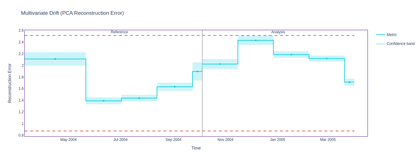
It seems that the reconstruction method didn't detect any significant drift in the dataset, as indicated by the absence of alerts in the figure above. One significant limitation of this method is its reliance on linear transformations to capture the underlying structure of the data. As a result, it may not accurately detect subtle or nonlinear changes in the dataset.

Let’s see if Domain Classifier picks up any drift.

# Initialize the Domain Classifier calculator
drift_classifier = nml.DomainClassifierCalculator(
    feature_column_names=feature_names,
    timestamp_column_name='Timestamp',
    chunk_size=1000
).fit(reference_data=reference_set)

# Calculate drift using the Domain Classifier
drift_classifier_results = drift_classifier.calculate(data=analysis_set)

# Visualize the drift detection results
figure2 = drift_classifier_results.plot()
figure2.show()

The Domain Classifier algorithm has detected various drifts, as shown below.

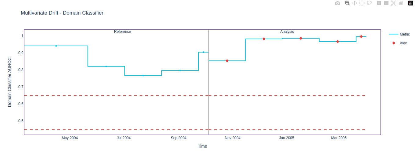
Figure 7: Domain Classifier Algorithm with chunk size = 1000

The reference period in the above result lies outside the threshold (unlike the result of the PCA reconstruction method). This implies that the classifier detects changes in the reference dataset, which should not happen. This highlights a significant limitation of the Domain Classifier method: its sensitivity to minor fluctuations. Generally, this method needs more data than the PCA reconstructor method to provide reliable results.

On increasing the chunk size to 10,000, the issue is resolved, and stable output is achieved.

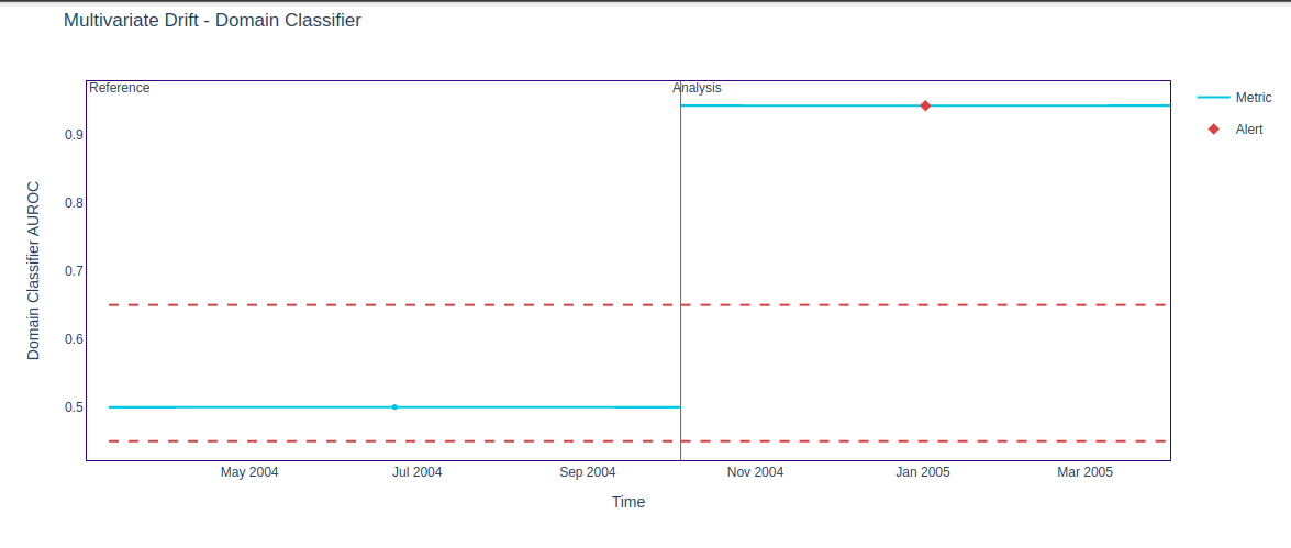
Figure 8: Domain Classifier Algorithm with chunk size = 10000

Larger chunk sizes even out the results and are less sensitive to minor variations, thereby providing stable scores. However, this also leads to a loss in granularity. Smaller chunks, on the other hand, mean more comparisons and possibly generate more false positives.

An alternative to changing the chunk size would be to tune hyperparameters such as n_estimators or threshold values. However, hyperparameter tuning can be more elaborate and time-consuming than simply tuning the chunk size.

💡

Note:

The fit method for both calculators is responsible for training the drift detection model, but they use different techniques: dimensionality reduction for DataReconstructionDriftCalculator and domain classification for DomainClassifierCalculator. We have discussed the underlying theory for both above.

The calculate method assesses drift differently based on the trained model: reconstruction error and the AUROC, respectively.

I simulated drift by changing the values of specific features, such as 'CO(GT)' and 'C6H6(GT)', by a factor of 0.8 since the dataset. This artificial drift injection will help showcase the functionality of our drift detection algorithms in identifying and quantifying changes within the dataset over time.

drifted_features = ['CO(GT)', 'C6H6(GT)']
drift_intensity = 0.8  
analysis_set_with_drift = analysis_set.copy()
analysis_set_with_drift[drifted_features] *= (1 + drift_intensity)

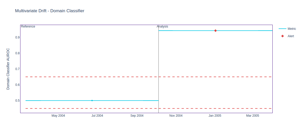
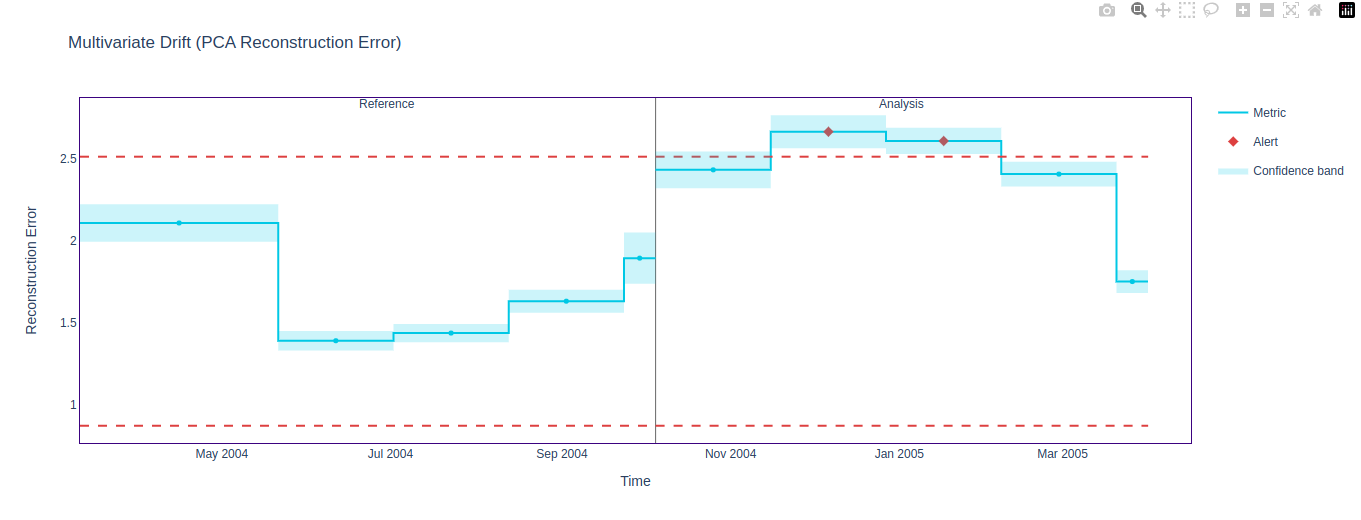
In the original dataset, we noted that the Data Reconstruction Drift Calculator did not detect drift as effectively as the Domain Classifier. The figures below show that the artificial drift that we injected was detected by both algorithms. The chunk size in this scenario is 10000.

Figure 9: Domain Classifier with injected drift.

Figure 10: PCA Reconstruction Algorithm with injected drift.

Summary

Each method has its own set of best practices and suitable use cases. The DataReconstructionDriftCalculator is more suitable for datasets with linear relationships, where the underlying structure can be effectively captured by eigenvectors. The DomainClassifierCalculator approach is more suitable for datasets with complex distributions.

It is important to be careful with feature selection, preprocessing and hyperparameter tuning.

This tabular comparison summarizes both the algorithms in a neat manner:

Characteristics	Data Reconstruction with PCA	Domain Classifier
Working Principle	Detect changes in the overall structure of the data	Assess dissimilarity between reference and analyzed datasets
Data Preprocessing	Address missing values, encode categorical features, scale data	Assign labels, concatenate datasets, encode categorical data
Model	Principal Component Analysis (PCA)	LightGBM classifier
Evaluation Metric	Reconstruction error	Cross-validated AUROC score
Limitations	It may not capture all types of drift and nonlinear changes.	Requires careful tuning and interpretation of AUROC scores. It is also sensitive to biases and errors during preprocessing.

Your model might face degradation for various other reasons. To learn more about how you can improve your machine-learning applications and how NannyML is just the solution for you, Schedule a Demo with the founders today!

Frequently Asked Questions

What is the main cause of model degradation in machine-learning applications?

Model degradation in machine learning is mainly caused by data drift, including covariate shift, where input feature distribution changes over time. This can lead to a significant drop in model performance. NannyML offers advanced drift detection methods to identify and address these shifts effectively, ensuring your models remain accurate and reliable.

How can I detect and mitigate covariate shifts in my machine-learning models?

Covariate Shift can be detected using univariate detection methods and multivariate detection methods. Data scientists can mitigate covariate shifts by re-sampling the training dataset to resemble the production(newer) data. Adversarial training also makes the models robust to distribution changes.

How do multivariate drift detection methods differ from univariate approaches?

Multivariate drift detection methods analyze changes in relationships between multiple features simultaneously, capturing complex data shifts. Univariate approaches focus on changes in individual feature distributions. Multivariate methods, like those offered by NannyML, provide a more comprehensive view, detecting subtle and interdependent shifts that univariate methods might miss.

Comparing Multivariate Drift Detection Algorithms on Real-World Data